Lab-10 RC Transient Circuits:

Name: Write down your name

Date: Date of report submission and date of lab performed

Learning Objectives:

Understand RC transient circuits.

Determine the RC time constant of a circuit through simulation, experiment, and analytically.

Understand by differentiating and integrating the RC circuits and how the performance is affected by frequency and the time constant.

Capacitive RC Circuit:

The capacitor has a wide range of applications in electronic circuits, some of which are energy storage, dc blocking, filtering, and timing. Thus, it is important for engineering students to understand electronic circuit with capacitor. This experiment is designed to familiarize the student with the simple transient response of two-element RC circuits, and the various methods for measuring and displaying these responses.

Charging of a Capacitor:

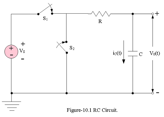
In normal operation, a capacitor charges part of the time and discharges at other times. Consider first the charging process. In the circuit of Figure 10.1, for t < 0, both of the switches are open and no energy is stored on the capacitor. We say that the initial conditions are zero, or \(V_0(0) = 0\). At time t = 0, switch \(S_1\) closes and the capacitor begins charging.

The capacitance, C, in Farad of a capacitor is related to charge, q and the voltage, v, across the capacitor is given by:

\[C = \frac{q}{v}~~~~(10.1)\] In deriving the circuit equation for a RC circuit, we will use the current/voltage relationship for a capacitor.

\[i_C(t)=\frac{dq}{dt}=C\frac{v_C(t)}{dt}~~~~(10.2)\] The current through the capacitor in Eq. (10.2) is proportional to the time derivative of the voltage across the capacitor. Applying KCL at the upper capacitor node (for t > 0) yields

\[i_C(t)+\frac{v_0(t)-V_S}{R}=0\] \[C\frac{dv_0(t)}{dt}+\frac{v_0(t)-V_S}{R}=0~~~~(10.3)\] The solution of this linear, constant-coefficient differential Eq. (10.3) is

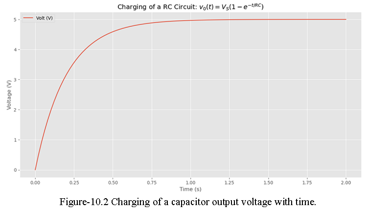
\[v_0(t)=V_S\left(1-e^{\frac{t}{RC}}\right)~~for~ t\gt 0~~~~(10.4)\] where \(\tau = RC\) in the circuit is known as the capacitive time constant.

As an example if we consider a \(C=100\times 10^{-6}~F,~ and ~R=2k\Omega\) with time RC time constant \(\tau = RC=0.2s\). A plot of Eq. (10.4) is shown in Figure 10.2 with the charging time span of 10RC (2.0s).

Discharging of a Capacitor:

Refering to Figure 10.1, that the capacitor has charged to a value \(V_S\) and at t = 0, switch \(S_1\) opens and switch \(S_2\) closes. With switch \(S_1\) opens the DC voltage source has been excluded,and using KCL at the same node as before we get,

\[C\frac{dv_0(t)}{dt}+\frac{v_0}{R}=0~~~t > 0~~~~(10.5)\] The solution of this linear, homogeneous, constant-coefficient differential equation is

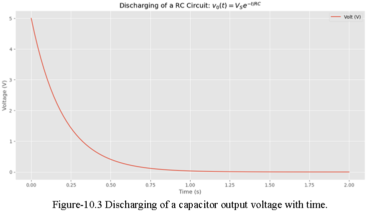
\[v_0(t)=V_Se^{-t/RC}~~~t > 0~~~~(10.6)\] A plot of Eq. (10.6) is shown in Figure 10.3 with the discharging time span of 10RC (2.0s).

RC Circuit Response to a Periodic Step-Voltage Excitation:

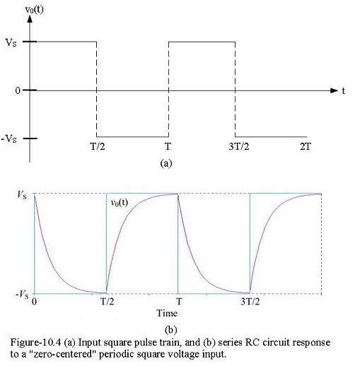
The oscilloscope can continuously display some portion of a periodic input waveform. A transient waveform, however, occurs only once, and is therefore not repetitive. It can be displayed conveniently only on an oscilloscope with memory. The oscilloscopes without memory, it is necessary to apply a repetitive “step” voltage to the input of the RC circuit to display the transient response of the circuit. A good approximation of the transient response may be obtained using a square-wave excitation since it is periodic and may be regarded as a series of positive and negative step voltages. For a periodic square wave with a reasonably long half-period (T/2 > 5\(\tau\)), the exponential rise and fall during a single half-period of the square wave will be practically complete. Thus, the oscilloscope display of a periodic step voltage will appear very similar to that of a single step input to the RC circuit, as is shown in Figure 10.4.

Design Criteria:

1. Consider R and \(V_S\) as design variables.

2. Let \(\tau\) (the period) be approximately 250 ms.

3. Use C = 0.1 \(\mu F\) in the RC design

4. Require \(V_0(10 ms)\) = 3.5 V and \(V_0(60 ms)\) = 0.1 V.

Hints:

Use the following general formula for the voltage stepping response of the first order system

\[V_0(t) = V_{inf} +(V(0) - V_{inf})*exp(-t/\tau)\], (\(\tau\) is the time constant)

Where: \(V_{inf}\) – steady state, asymptotic voltage,

V(0) – initial output voltage

\(V(0) - V_{inf}\) – transient part, dies out after “sufficient” time (practically sufficient time means \(~ 3\tau\) to \(5\tau\))

In this case (see Figure 10.4) \(V_{inf} = 0\), and the equation above reduces to \(V_0(t) = V(0)*exp(-t/\tau)\).

Finally, after substituting conditions 4) into the last equation and recognizing that V(0) = \(2*V_S\) (convince yourself that this holds true), it follows \(3.5 = 2*V_S*exp(-10 ms/\tau)\) and \(0.1 = 2*V_S*exp(-60 ms/\tau)\) The last two equations can now be solved for \(V_S\) and \(\tau\).

Sketch the circuit and record the calculations and results, including plots of $V_{in} vs. V_{out} with the relevant values indicated by the cursors.

Using L= 330 mH, design and sketch an RL circuit with the same specifications indicated above. Remember \(\tau\)=L/R for an RL circuit

to be continued…….