Chapter 9 Magnetic Fields Due to Currents

Learning Objectives:

In this chapter you will basically learn:

\(\bullet\) Learn that for a given point near a wire and a given current-element in the wire, how to determine the magnitude and direction of the magnetic field due to that element.

\(\bullet\) Learn the the direction of the field vector using a right-hand rule for a point to one side of a long straight wire carrying current.

\(\bullet\) Learn the Biot–Savart law to find the magnetic field set up at the point by the current.

\(\bullet\) Learn how parallel currents attract each other, and antiparallel currents repel each other.

\(\bullet\) Learn how to apply Ampere’s law, for determining the algebraic sign of an encircled current using a right-hand rule .

\(\bullet\) Learn how to apply Ampere’s law to a long straight wire with current, to find the magnetic field magnitude inside and outside the wire.

\(\bullet\) Learn how to apply Ampere’s law to find the magnetic field inside a solenoid.

\(\bullet\) Learn what is a solenoid and how its internal magnetic field B, the current i, and the number of turns per unit length n of the solenoid are related.

\(\bullet\) Learn how to apply Ampere’s law to find the magnetic field inside a toroid.

\(\bullet\) Learn what is a toroid and how its internal magnetic field B, the current i, the radius r, and the total number of turns N are related.

\(\bullet\) Learn how in a current-carrying coil, the dipole moment magnitude \(\mu\) and the coil’s current i, number of turns N, and area per turn A are related.

\(\bullet\) Learn how in a point along the central axis, magnetic field magnitude B, the magnetic dipole moment \(\mu\), and the distance z from the center of the coil are related.

9.1 Magnetic Fields Due to Currents:

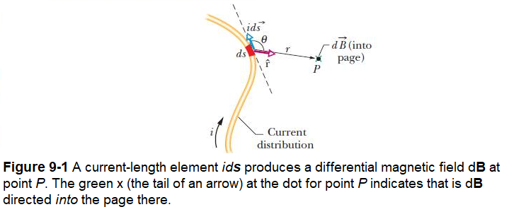
The magnitude of the field \(d\vec B\) produced at point P at distance r by a current-length element \(id\vec s\) turns out to be

\[\begin{equation} dB = \frac{\mu_0}{4\pi}\frac{ids~sin\theta}{r^2} \tag{9.1} \end{equation}\]

where \(\theta\) is the angle between the directions of \(d\vec s\) and \(\hat r\), a unit vector that points from ds toward P. Symbol \(\mu_0\) is a constant, called the permeability constant, whose value is defined to be exactly

\[\begin{equation} \mu_0=4\pi\times10^{-7}~\frac{T\cdot m}{A}\approx1.26\times10^{-6}\frac{T\cdot m}{A} \tag{9.2} \end{equation}\]

The direction of \(d\vec B\), shown as being into the page in Fig. 9-1, is that of the cross product \(d\vec s\times \hat r\).We can therefore write Eq. 9-1 in vector form as

\[\begin{equation} d\vec B =\frac{\mu_0}{4\pi}\frac{id\vec s\times\hat r}{r^2}~~~(Biot–Savart~law) \tag{9.3} \end{equation}\]

This vector equation and its scalar form, Eq. 9-1, are known as the law of Biot and Savart. The law, which is experimentally deduced, is an inverse-square law. We shall use this law to calculate the net magnetic field produced at a point by various distributions of current.

9.2 Magnetic Field Due to a Current in a Long Straight Wire:

Figure 9-2, shows a straight wire of infinite length, for which we want to find the field \(\vec B\) at point P, a perpendicular distance R from the wire. The magnitude of the differential magnetic field produced at P by the current-length element \(id\vec s\) located a distance r from P is given by Eq. 9-1:

\[\begin{equation} dB = \frac{\mu_0}{4\pi}\frac{ids~sin\theta}{r^2} \tag{9.4} \end{equation}\]

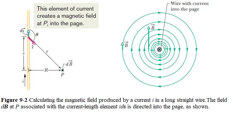
The direction of in Fig. 9-2 is that of the vector \((d\vec s\times \vec r)\), which is directly into the page. We can find the magnitude of the magnetic field produced at P by the current-length elements in the upper half of the infinitely long wire by integrating dB in Eq. 9-1 from 0 to \(\infty\). Similarly, the magnetic field produced by the lower half of the wire is exactly the same as that produced by the upper half. To find the magnitude of the total magnetic field \(\vec B\) at P, we need only multiply the result of our integration by 2. We get

\[\begin{equation} B=2\int_{0}^{\infty}dB=\frac{\mu_0i}{2\pi}\int_{0}^{\infty}\frac{sin\theta~ds}{r^2} \tag{9.5} \end{equation}\]

The variables \(\theta\), s, and r in this equation are not independent; Fig. 9-2 shows that they are related by

\(r=\sqrt {s^2+R^2}\) and \(sin\theta=sin(\pi-\theta)=\frac{R}{\sqrt {s^2+R^2}}\).

Using standard integral \(\int\frac{dx}{({x^2+a^2})^\frac{3}{2}}=\frac{x}{ a^2\sqrt {(x^2+a^2)}}\), we can get

\[\begin{equation} B =\frac{\mu_0i}{2\pi}\int_{0}^{\infty}\frac{R~ds}{(s^2+R^2)^{3/2}}=\frac{\mu_0i}{2\pi R} \left[\frac{s}{\sqrt{s^2+R^2}}\right]_{0}^{\infty}=\frac{\mu_0i}{2\pi R} \tag{9.6} \end{equation}\]

Note that the magnetic field at P due to either the lower half or the upper half of the infinite wire in Fig. 9-2 is half this value; that is,

\[\begin{equation} B =\frac{\mu_0i}{4\pi R}~~~(semi-infinite~straight~wire). \tag{9.7} \end{equation}\]

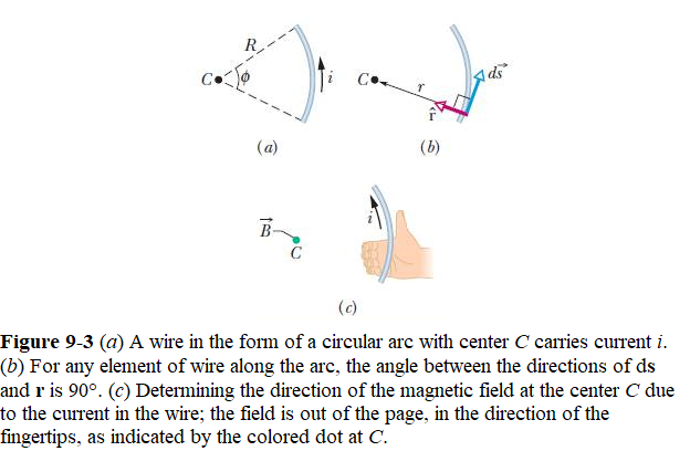
Magnetic Field Due to a Current in a Circular Arc of Wire: Figure 9-3a shows such an arc-shaped wire with central angle \(\phi\), radius R, and center C, carrying current i. At C, each current-length element \(id\vec s\) of the wire produces a magnetic field of magnitude dB given by Eq. 9-4. Moreover, as Fig. 9-3b shows, no matter where the element is located on the wire, the angle \(\theta\) between the vectors \(d\vec s\) and \(\vec r\)is \(90^0\); also, r = R. Thus, by substituting R for r and \(90^0\) for \(\theta\) in Eq. 9-4, we obtain

\[\begin{equation} dB = \frac{\mu_0}{4\pi}\frac{ids}{r^2} \tag{9.8} \end{equation}\]

Now in Eq. 9-8 we substitute \(ds = Rd\phi\) and then by integrating we get an expression for an arbitrary arc of a circular current carrying ring as follows:

\[B=\int dB=\int_{0}^{\phi}\frac{\mu_0}{4\pi}\frac{iRd\phi}{R^2}= \frac{\mu_0i}{4\pi R}\int_{0}^{\phi}d\phi\]

Integrating over the circular arc, we get

\[\begin{equation} B=\frac{\mu_0i}{4\pi R}\int_{0}^{\phi}d\phi=\frac{\mu_0i\phi}{4\pi R}~~~(at~center~of~ circular~arc). \tag{9.9} \end{equation}\]

As an example, for a full circular current carrying conductor we can find the magnetic field at the center by substituting \(2\pi\) rad for \(\phi\) in Eq. 9-9, we get

\[\begin{equation} B=\frac{\mu_0i2\pi}{4\pi R}= \frac{\mu_0i}{2R}~~~(at~center~of~ full~circle). \tag{9.10} \end{equation}\]

9.3 Force Between Two Parallel Currents:

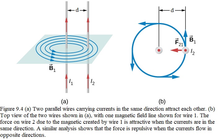
The force between two long, straight, and parallel conductors separated by a distance d can be found by applying the result in Eq. 8-20 \((\vec F_B = i\vec L \times \vec B)\). Figure 9.4 shows the wires, their currents, the magnetic field created by wire 1, and the force it exerts on wire 2 (call the force \(\vec F_{21}\). The field due to \(i_1\) at a distance d is

\[\begin{equation} \vec F_{21}= i_2\vec L \times \vec B_1 \tag{9.11} \end{equation}\]

\[\begin{equation} \vec F_{21}= i_2LB_1\sin90^0=\frac{\mu_0Li_1i_2}{2\pi d} \tag{9.12} \end{equation}\]

The direction of \(\vec F_{21}\) is the direction ofthe cross-product of \(\vec L\times \vec B_1\) and is directed towards the wire 1, as shown in Fig. 9-4.

9.4 Ampere’s Law:

Over an arbitrary closed path,

\[\begin{equation} \oint\vec{\mathbf{B}}\cdot d\vec{\mathbf{s}}=\mu_0i_{enc}~~~(Ampere’s~Law) \tag{9.13} \end{equation}\]

The line integral in this equation is evaluated around a closed loop called an Amperian loop. The current i on the right side is the net current encircled by the loop.

EXAMPLE 9.1 Using Ampère’s law to calculate the magnetic field due to a steady current i in an infinitely long, thin, straight wire as shown in Figure 9.5.

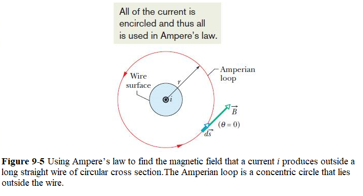
Figures shows an infinitely long, thin, straight wire with the current directed into the page. The radial and polar components of magnetic field, \(B_r\) and \(B_{\Theta}\) respectively, are shown at arbitrary points on a circle of radius r centered on the wire. The possible components of the magnetic field B due to a current i, which is directed into the page. The radial component is zero because the angle between the magnetic field and the path is at a right angle.

Solution: Over this path \(\vec B\) is constant and is parallel to \(d\vec s\), so

\[\oint\vec B\cdot d\vec s = B_{\theta}\oint ds = B_{\theta}(2\pi r)\]

Thus Ampère’s law reduces to

\[B_{\theta}(2\pi r)=\mu_0i\]

Finally, since \(B_{\theta}\) is the only component of \(\vec B\) we can drop the subscript and write

\[B=\frac{\mu_0i}{2\pi r}~~~(Answer)\]

This agrees with the result we got using Biot-Savart law in Eq.9-6.

Magnetic Field Inside a Long Straight Wire with Current: Figure 9-6 shows the cross section of a long straight wire of radius R that carries a uniformly distributed current i directly out of the page.

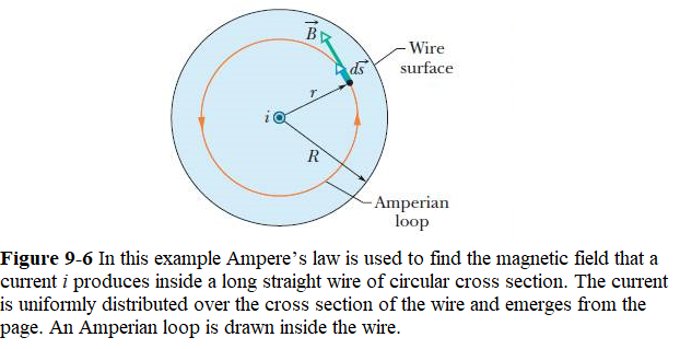
The magnetic field created by the uniform current must be cylindrically symmetrical. To calculate the magnetic field at points inside the wire, we can apply an Amperian loop of radius r, as shown in Fig. 9-6, where now \(r < R\). Magnetic field \(\vec B\) (Eq. 9-13) is tangent to the loop, as shown; so the left side of Ampere’s law yields

\[\begin{equation} \oint\vec B\cdot d\vec s = \oint B~cos\theta~ ds=B\oint ds=B(2\pi r) \tag{9.14} \end{equation}\]

The current \(i_{enc}\) encircled by the loop is proportional to the area encircled by the loop; that is,

\[\begin{equation} i_{enc}=\frac{\pi r^2}{\pi R^2} \tag{9.15} \end{equation}\]

Now applying Ampere’s law we can find the magnetic inside the conductor

\[B(2\pi r) = \mu_0 i\frac{\pi r^2}{\pi R^2}\]

\[\begin{equation} B = \left(\frac{\mu_0 i}{2\pi R^2}\right)r~~~(magnetic~field~inside~the~straight~wire). \tag{9.16} \end{equation}\]

Thus, inside the wire, the magnitude B of the magnetic field is proportional to r , is zero at the center, and is maximum at r = R (at the surface).

9.5 Solenoids:

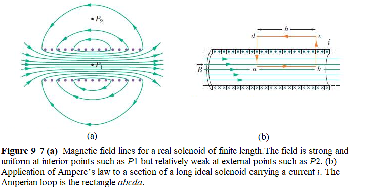
Figure 9-7-a shows the lines of for a real solenoid and Figure 9-7-b shows an ideal solenoid. The spacing of these lines in the central region shows that the field inside the coil is fairly strong and uniform over the cross section of the coil. The external field, however, is relatively weak.

Let us now apply Ampere’s law,

\[\begin{equation} \oint\vec{\mathbf{B}}\cdot d\vec{\mathbf{s}}=\mu_0i_{enc}~~~(Ampere’s~Law) \tag{9.17} \end{equation}\]

to the ideal solenoid of Fig. 9-7 (b), where \(\vec B\)is uniform within the solenoid and zero outside it, using the rectangular Amperian loop abcda. We write \(\oint\vec{\mathbf{B}}\cdot d\vec{\mathbf{s}}\)as the sum of four integrals, one for each loop segment:

\[\begin{equation} \oint\vec{\mathbf{B}}\cdot d\vec{\mathbf{s}}= \int_{a}^{b}\vec{\mathbf{B}}\cdot d\vec{\mathbf{s}} + \int_{b}^{c}\vec{\mathbf{B}}\cdot d\vec{\mathbf{s}} +\int_{c}^{d}\vec{\mathbf{B}}\cdot d\vec{\mathbf{s}} +\int_{d}^{a}\vec{\mathbf{B}}\cdot d\vec{\mathbf{s}} \tag{9.18} \end{equation}\]

The first integral on the right of Eq. 9-18 is Bh, where B is the magnitude of the uniform field \(\vec B\)inside the solenoid and h is the (arbitrary) length of the segment from a to b. The second and fourth integrals are zero because for every element ds of these segments \(\vec B\), either is perpendicular to ds or is zero, and thus the product \(\vec B.d\vec s\)is zero.The third integral, which is taken along a segment that lies outside the solenoid, is zero because B = 0 at all external points. Thus, \(\vec{\mathbf{B}}\cdot d\vec{\mathbf{s}}\)for the entire rectangular loop has the value Bh.

The net current \(i_{enc}\) encircled by the rectangular Amperian loop in Fig. 9-7 is not the same as the current i in the solenoid windings because the windings pass more than once through this loop. Let n be the number of turns per unit length of the solenoid; then the loop encloses nh turns and \[i_{enc}=i(nh)\] Ampere’s law then gives us \[Bh=\mu_0 inh\] \[\begin{equation} B = \mu_0 in~~~(ideal~solenoid). \tag{9.19} \end{equation}\]

An application of solenoid is the a magnetic resonance imaging (MRI). In an MRI scan, the person lies down on a table that is moved into the center of a large solenoid that can generate very high magnetic fields that is being created by passing high currents flowing through the superconducting wires. The large magnetic field is used to change the spin of protons in the patient’s body. The time it takes for the spins to align or relax (return to original orientation) is a signature of different tissues that can be analyzed to see if the structures of the tissues is normal (Figure 9.8).

EXAMPLE 9.2

A solenoid has 300 turns wound around a cylinder of diameter \(1.20~\mathrm{cm}\) and length \(14.0~\mathrm{cm}\). If the current through the coils is \(0.410~\mathrm{A}\), what is the magnitude of the magnetic field inside and near the middle of the solenoid?

Solution: The number of turns per unit length is

\[n=\frac{300~\mathrm{turns}}{0.140~\mathrm{m}}=2.14\times10^3~\mathrm{turns/m}.\]

The magnetic field produced inside the solenoid is

\[\begin{eqnarray*}B&=&\mu_0nI=(4\pi\times10^{-7}~\mathrm{T}\cdot\mathrm{m/A})(2.14\times10^3~\mathrm{turns/m})(0.410~\mathrm{A})\\&=&1.10\times10^{-3}~\mathrm{T}.\end{eqnarray*}\]

9.6 Toroids:

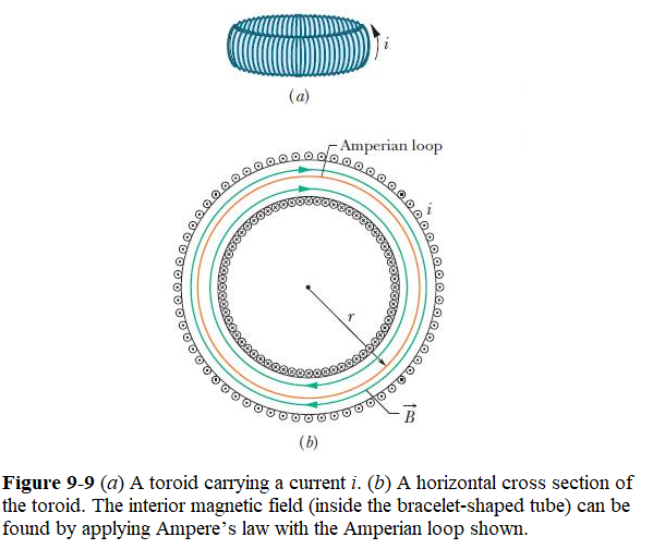
Figure 9-9a shows a toroid, which we may describe as a (hollow) solenoid that has been curved until its two ends meet, forming a sort of hollow bracelet.What magnetic field is set up inside the toroid (inside the hollow of the bracelet)? We can find out from Ampere’s law and the symmetry of the bracelet.

From the symmetry, we see that the lines of \(\vec B\) form concentric circles inside the toroid, directed as shown in Fig. 9-9b. Let us choose a concentric circle of radius r as an Amperian loop and traverse it in the clockwise direction. Using Ampere’s law we get

\[(B)(2\pi r)=\mu_0iN\] \[\begin{equation} B = \frac{\mu_0 iN}{2\pi}\frac{1}{r}~~~(Toroid). \tag{9.20} \end{equation}\]

In Eq. 9-20,one can see that B is not constant over the cross section of a toroid.

9.7 A Current-Carrying Coil as a Magnetic Dipole:

In the last few sections we studied the magnetic fields produced by current in a long straight wire, a solenoid, and a toroid. We found how magnetic dipole moment resulted in a current carrying loop in section 8.9, Eq. 8-24. We also briefly discussed in Example 8.2 how torque \(\vec\tau\) tau can be created if we place it in an external magnetic field \(\vec B\),

\[\begin{equation} \vec\tau = \vec\mu \times \vec B \tag{9.21} \end{equation}\]

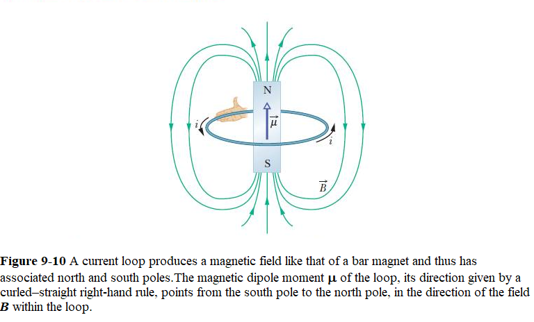
In Eq. 9-21, \(\vec\mu\) is the magnetic dipole moment of the coil and has the magnitude NiA, where N is the number of turns, i is the current in each turn, and A is the area enclosed by each turn. The direction of the magnetic dipole moment \(\vec\mu\)is shown in Figure 9-10, can be found by applying right-handed rule placing your fingers of your right hand curl around it in the direction of the current; with your extended thumb then points in the direction of the dipole moment \(\vec\mu\) as shown in Figure 9-10.

The magnetic field element \(d\vec B\) has two components, \(dB_{\|}\) along the axis of the loop and \(dB_{\perp}\) perpendicular to this axis. From the symmetry, the vector sum of all the perpendicular components \(dB_{\perp}\) due to all the loop elements ds is zero. This leaves only the axial (parallel) components \(dB_{\|}\), and we have

\[B=\int dB_{\|}\]

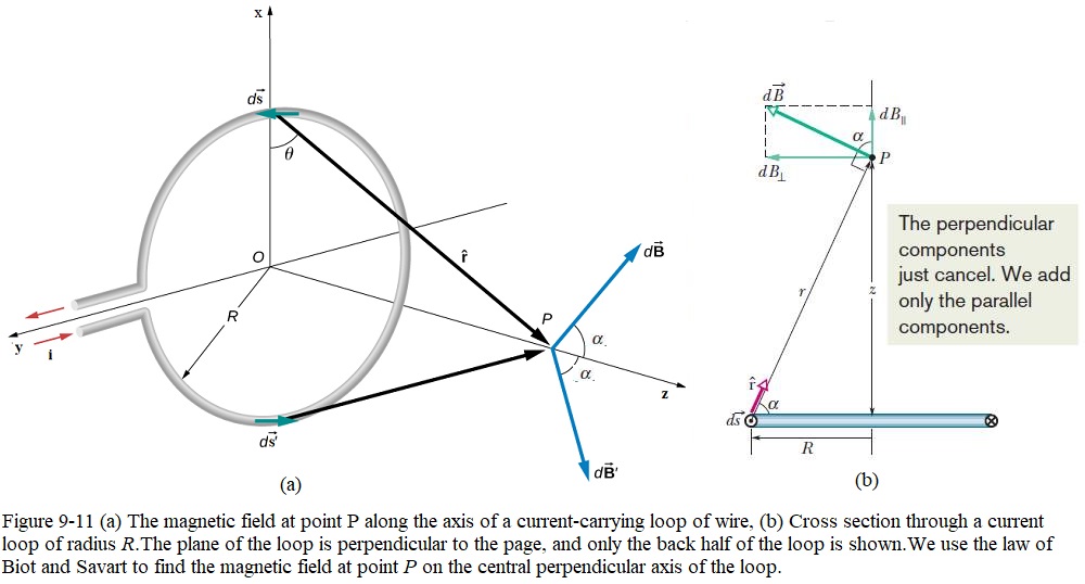
The element \(d\vec s\) as shown in in Fig. 9-11, the law of Biot and Savart (Eq. 9-3) tells us that the magnetic field at distance r is

\[dB = \frac{\mu_0}{4\pi}\frac{ids\sin90^0}{r^2}\]

\[dB_{\|} = dB\cos\alpha\]

\[\begin{equation} dB_{\|}=\frac{\mu_0i~\cos\alpha~ ds}{4~\pi~r^2} \tag{9.22} \end{equation}\]

Figure 9-11 shows that r and \(\alpha\) are related to each other. Let us express each in terms of the variable z, the distance between point P and the center of the loop. The relations are

\[\begin{equation} r=\sqrt{R^2+z^2} \tag{9.23} \end{equation}\]

and

\[\begin{equation} \cos\alpha=\frac{R}{r}=\frac{R}{\sqrt{R^2+z^2}} \tag{9.24} \end{equation}\]

Substituting Eqs. 9-23 and 9-24 into Eq. 9-22, we find

\[dB_{\|}=\frac{\mu_0iR}{4\pi(R^2+z^2)^{3/2}}\] \[B=\int dB_{\|}=\frac{\mu_0iR}{4\pi(R^2+z^2)^{3/2}}\int ds\] or, because \(\int~ds\)is simply the circumference \(2\pi R\) of the loop,

\[\begin{equation} B(z)=\frac{\mu_0iR^2}{2(R^2+z^2)^{3/2}}. \tag{9.25} \end{equation}\]

Solved Problems Magnetic Fields Due to Currents

1. [7] In Fig. 29-39, two circular arcs have radii a = 13.5 cm and b = 10.7 cm, subtend angle \(\theta=74^\circ\), carry current i = 0.411 A, and share the same center of curvature P. What are the (a) magnitude and (b) direction (into or out of the page) of the net magnetic field at P?

2. [9] Two long straight wires are parallel and 8.0 cm apart. They are to carry equal currents such that the magnetic field at a point halfway between them has magnitude 300 mT. (a) Should the currents be in the same or opposite directions? (b) How much current is needed?

3. [11] In Fig. 29-42, two long straight wires are perpendicular to the page and separated by distance \(d_1\) = 0.75 cm. Wire 1 carries 6.5 A into the page. What are the (a) magnitude and (b) direction (into or out of the page) of the current in wire 2 if the net magnetic field due to the two currents is zero at point P located at distance \(d2\) = 1.50 cm from wire 2?

4. [13] In Fig. 29-44, point \(P_1\) is at distance R = 13.1 cm on the perpendicular bisector of a straight wire of length L = 18.0 cm carrying current i = 58.2 mA. (Note that the wire is not long.) What is the magnitude of the magnetic field at \(P_1\) due to i?

5. [21] Figure 29-49 shows two very long straight wires (in cross section) that each carry a current of 4.00 A directly out of the page. Distance \(d_1\) = 6.00 m and distance \(d_2\) = 4.00 m. What is the magnitude of the net magnetic field at point P, which lies on a perpendicular bisector to the wires?

6. [31] In Fig. 29-59, length a is 4.7 cm (short) and current i is 13 A. What are the (a) magnitude and (b) direction (into or out of the page) of the magnetic field at point P?

Section 9-2 Force Between Two Parallel Currents

7. [35] Figure 29-63 shows wire 1 in cross section; the wire is long and straight, carries a current of 4.00 mA out of the page, and is at distance \(d_1\) = 2.40 cm from a surface. Wire 2, which is parallel to wire 1 and also long, is at horizontal distance \(d_2\) = 5.00 cm from wire 1 and carries a current of 6.80 mA into the page. What is the x component of the magnetic force per unit length on wire 2 due to wire 1?

Section 9-3 Ampere’s Law

8. [43] Figure 29-67 shows a cross section across a diameter of a long cylindrical conductor of radius a = 2.00 cm carrying uniform current 170 A.What is the magnitude of the current’s magnetic field at radial distance (a) 0, (b) 1.00 cm, (c) 2.00 cm (wire’s surface), and (d) 4.00 cm?

Section 9-4 Solenoids and Toroids

9. [49] A toroid having a square cross section, 5.00 cm on a side, and an inner radius of 15.0 cm has 500 turns and carries a current of 0.800 A. (It is made up of a square solenoid—instead of a round one as in Fig. 29-17—bent into a doughnut shape.) What is the magnetic field inside the toroid at (a) the inner radius and (b) the outer radius?

10. [51] A 200-turn solenoid having a length of 25 cm and a diameter of 10 cm carries a current of 0.29 A. Calculate the magnitude of the magnetic field inside the solenoid.

11. [53] A long solenoid has 100 turns/cm and carries current i.An electron moves within the solenoid in a circle of radius 2.30 cm perpendicular to the solenoid axis. The speed of the electron is 0.0460c (c = speed of light). Find the current i in the solenoid.

12. [55] A long solenoid with 10.0 turns/cm and a radius of 7.00 cm carries a current of 20.0 mA. A current of 6.00A exists in a straight conductor located along the central axis of the solenoid. (a) At what radial distance from the axis will the direction of the resulting magnetic field be at \(45^\circ\) to the axial direction? (b) What is the magnitude of the magnetic field there?

Section 9-5 A Current-Carrying Coil as a Magnetic Dipole

13. [62] In Fig. 29-75, current i = 56.2 mA is set up in a loop having two radial lengths and two semicircles of radii a = 5.72 cm and b ! 9.36 cm with a common center P. What are the (a) magnitude and (b) direction (into or out of the page) of the magnetic field at P and the (c) magnitude and (d) direction of the loop’s magnetic dipole moment?

Problems Magnetic Fields Due to Currents

1. [8] In Fig. 29-40, two semicircular arcs have radii \(R_2\) = 7.80 cm and \(R_1\) = 3.15 cm, carry current i = 0.281 A, and have the same center of curvature C. What are the (a) magnitude and (b) direction (into or out of the page) of the net magnetic field at C?

2. [10] In Fig. 29-41, a wire forms a semicircle of radius R = 9.26 cm and two (radial) straight segments each of length L = 13.1 cm. The wire carries current i = 34.8 mA. What are the (a) magnitude and (b) direction (into or out of the page) of the net magnetic field at the semicircle’s center of curvature C?

3. [12] In Fig. 29-43, two long straight wires at separation d = 16.0 cm carry currents \(i_1\) = 3.61 mA and \(i_2\) = 3.00\(i_1\) out of the page. (a) Where on the x axis is the net magnetic field equal to zero?

2. If the two currents are doubled, is the zero-field point shifted toward wire 1, shifted toward wire 2, or unchanged?

4. [24] Figure 29-52 shows, in cross section, four thin wires that are parallel, straight, and very long. They carry identical currents in the directions indicated. Initially all four wires are at distance d = 15.0 cm from the origin of the coordinate system, where they create a net magnetic field \(\vec B\). (a) To what value of x must you move wire 1 along the x axis in order to rotate counterclockwise by \(30^\circ\)? (b) With wire 1 in that new position, to what value of x must you move wire 3 along the x axis to rotate by \(30^\circ\) back to its initial orientation?

5. [33] Figure 29-61 shows a cross section of a long thin ribbon of width w = 4.91 cm that is carrying a uniformly distributed total current i = 4.61 \(\mu A\) into the page. In unit-vector notation, what is the magnetic field \(\vec B\) at a point P in the plane of the ribbon at a distance d = 2.16 cm from its edge? (Hint: Imagine the ribbon as being constructed from many long, thin, parallel wires.)

Section 9-2 Force Between Two Parallel Currents

6. [41] In Fig. 29-66, a long straight wire carries a current \(i_1\) = 30.0 A and a rectangular loop carries current \(i_2\) = 20.0 A. Take the dimensions to be a = 1.00 cm, b = 8.00 cm, and L = 30.0 cm. In unitvector notation, what is the net force on the loop due to \(i_1\)?

Section 9-3 Ampere’s Law

7. [48] In Fig. 29-71, a long circular pipe with outside radius R ! 2.6 cm carries a (uniformly distributed) current i = 8.00 mA into the page. A wire runs parallel to the pipe at a distance of 3.00R from center to center. Find the (a) magnitude and (b) direction (into or out of the page) of the current in the wire such that the net magnetic field at point P has the same magnitude as the net magnetic field at the center of the pipe but is in the opposite direction.

Section 9-4 Solenoids and Toroids

8. [50] A solenoid that is 95.0 cm long has a radius of 2.00 cm and a winding of 1200 turns; it carries a current of 3.60 A. Calculate the magnitude of the magnetic field inside the solenoid.

9. [52] A solenoid 1.30 m long and 2.60 cm in diameter carries a current of 18.0 A. The magnetic field inside the solenoid is 23.0 mT. Find the length of the wire forming the solenoid.

10. [54] An electron is shot into one end of a solenoid. As it enters the uniform magnetic field within the solenoid, its speed is 800 m/s and its velocity vector makes an angle of \(30^\circ\) with the central axis of the solenoid. The solenoid carries 4.0 A and has 8000 turns along its length. How many revolutions does the electron make along its helical path within the solenoid by the time it emerges from the solenoid’s opposite end? (In a real solenoid, where the field is not uniform at the two ends, the number of revolutions would be slightly less than the answer here.)

Section 9-5 A Current-Carrying Coil as a Magnetic Dipole

11. [56] Figure 29-72 shows an arrangement known as a Helmholtz coil. It consists of two circular coaxial coils, each of 200 turns and radius R = 25.0 cm, separated by a distance s = R.The two coils carry equal currents i = 12.2 mA in the same direction. Find the magnitude of the net magnetic field at P, midway between the coils.