Chapter 4 Electric Potential

Learning Objectives:

In this chapter you will basically learn:

\(\bullet\) Learn how a charged particle sets up an electric potential V, which is a scalar quantity that can be positive or negative depending on the sign of the object’s charge.

\(\bullet\) Learn how to make the relationship between the electric potential V, the electric charge q, and the electric potential energy U.

\(\bullet\) Learn how to convert energies in joules to electron-volts and vice versa.

\(\bullet\) Learn the relationships between the change \(\Delta V\) in the potential, the particle’s charge q, the change \(\Delta U\) in the potential energy, and the work W done by the electric force.

\(\bullet\) Learn the path independence of the work done by the electric force.

\(\bullet\) Learn how change in electric potential \(\Delta V\) is related to the change in the particle’s kinetic energy \(\Delta K\).

\(\bullet\) Learn an equipotential surface and how it is related to the direction of the electric field, draw equipotential lines for a charged particle..

\(\bullet\) Learn the potential V at any given point due to an electric dipole, and express in terms of the magnitude p of the dipole moment or the product of the charge separation d and the magnitude q of either charge.

\(\bullet\) Learn the potential due to a continuous charge distribution.

\(\bullet\) Learn how in a uniform electric field, the magnitude of \(\vec E\) and the separation \(\Delta x\) and potential difference \(\Delta V\) are related between adjacent equipotential lines.

\(\bullet\) Learn the electric potential energy of a system of charged particles.

\(\bullet\) Learn the potential of a charged isolated conductor.

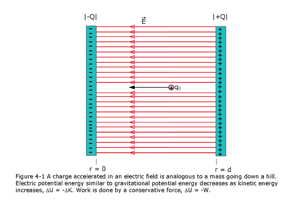
4.1 Electric Potential and Electric Potential Energy:

The electrical potential is analogous to an object being accelerated by a gravitational field. A test positive charge is placed in an electrical field its electric potential energy gets converted into kinetic energy. When a free positive charge q is accelerated by an electric field, it is given kinetic energy (Figure 3.1.1). Let us explore the work done on a charge q by the electric field in this process, so that we may develop a definition of electric potential energy. In chapter 9 , we defined potential energy when a conservative force does work W on a particle, the change \(\Delta U\) in the potential energy occur as given by

\[\begin{equation} \Delta U = -W. \tag{4.1} \end{equation}\]

If the particle moves from point 0 to point R, the change in the potential energy of the system is

\[\begin{equation} \Delta U = -W = -\int_{0}^{R}\vec F(\vec r).d\vec r = -\int_{0}^{R} q_0\vec E(\vec r).d\vec r \tag{4.2} \end{equation}\]

With potential energy to be zero at infinity we can write

\[\begin{equation} U = -W \tag{4.3} \end{equation}\]

Electric potential V at P as shown in Figure 24-2 in terms of the work done by the electric force and the resulting potential energy:

\[\begin{equation} V = -\frac{W_{\infty}}{q_0}= \frac{U}{q_0} \tag{4.4} \end{equation}\]

A charged particle with, say, charge q at a point where V exits, we can immediately find the potential energy of the configuration:

\[\begin{equation} U = qV \tag{4.5} \end{equation}\]

SI Units for Potential. The SI unit for potential that follows from Eq. 4-2 is the joule per coulomb. This combination occurs so often that a special unit, the volt (abbreviated V), is used to represent it.Thus,

1 volt = 1 joule per coulomb.

With two unit conversions, we can now switch the unit for electric field from newtons per coulomb to a more conventional unit:

\(\frac{1~N}{C}=\left(\frac{1~N}{C}\right)\left(\frac{1~V}{1~J/C}\right)\left(\frac{1~J}{1~N-m}\right) = \frac{1~V}{m}\)

If we move a charge from an initial point i to a second point f in the electric field of a charged object, the electric potential changes by \(\Delta = V_f - V_i\)

\[\begin{equation} \Delta U = q\Delta V = q(V_f-V_i) \tag{4.6} \end{equation}\]

We can relate the potential energy change \(\Delta U\) to the work W done by the electric force as the particle moves from i to f is given by:

\[\begin{equation} W = -\Delta U (work,~conservative~force) \tag{4.7} \end{equation}\]

We can relate that work to the change in the potential by substituting from Eq. 4-4:

\[\begin{equation} W = -\Delta U = -q\Delta V = -q(V_f - V_i) \tag{4.8} \end{equation}\]

Electron-volts. In atomic and subatomic physics, energy measures in the SI unit of joules often require awkward powers of ten.

A convenient non-SI unit is used in electron-volt (eV), in atomic and subatomic physics instead of using Joules. This is defined to the work required to move a single elementary charge e (such as that of an electron or proton) through a potential difference \(\Delta V\) of exactly one volt. From Eq. 4-6, we see that the magnitude of this work is \(q\Delta V\).Thus,

\[\begin{equation} 1~eV = e(1~V) = (1.6\times 10^{-19}C)(1J/C) = 1.6\times 10^{-19}J \tag{4.9} \end{equation}\]

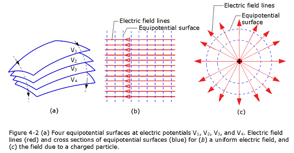
4.2 Equipotential Surfaces:

Figure 4-2a shows a family of equipotential surfaces associated with the electric field due to some distribution of charges. Figure 4-2b shows electric field lines and cross sections of the equipotential surfaces for a uniform electric field and Figure 4-2c for the field associated with a charged particle.

4.3 Calculating the Potential from the Field:

Consider an arbitrary electric field, represented by the field lines in Fig. 4-3, and a positive test charge \(q_0\) that moves along the path shown from point i to point f. At any point on the path, an electric force \(q_0\vec E\) acts on the charge as it moves through a differential displacement \(d\vec s\).

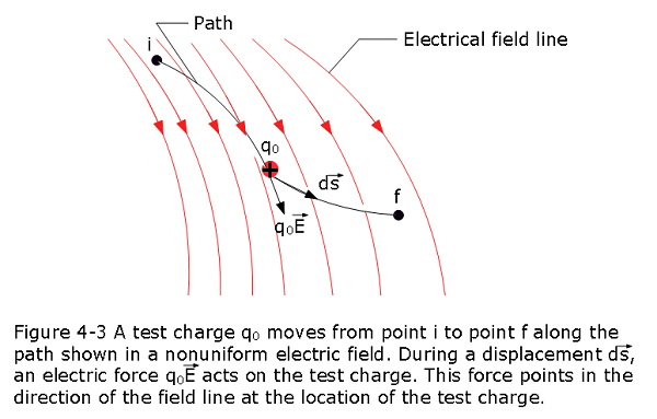
\[\begin{equation} dW = \vec F.d\vec s \tag{4.10} \end{equation}\]

\[\begin{equation} dW = q_0\vec E.d\vec s \tag{4.11} \end{equation}\]

\[\begin{equation} W = q_0 \int_{i}^{f} \vec E.d\vec s \tag{4.12} \end{equation}\]

If we substitute the total work Wfrom Eq. 4-10 into Eq. 4-6, we find

\[\begin{equation} V_f-V_i = -\int_{i}^{f} \vec E.d\vec s \tag{4.13} \end{equation}\]

Equation 4-11 allows us to calculate the difference in potential between any two points in the field. If we set potential \(V_i=0\), then Eq. 4-11 becomes

\[\begin{equation} V = -\int_{i}^{f} \vec E.d\vec s \tag{4.14} \end{equation}\]

in Equation 4-12 we have dropped the subscript f on \(V_f\).

Example Problem 4.01:

Figure 4-4a shows two points i and f in a uniform electric field. The points lie on the same electric field line (not shown) and are separated by a distance d. Find the potential difference \(V_f - V_i\) by moving a positive test charge \(q_0\) from i to f along the path shown, which is parallel to the field direction. (b) Now find the potential difference \(V_f - V_i\) by moving the positive test charge \(q_0\) from i to f along the path icf shown in Fig. 4-4b.

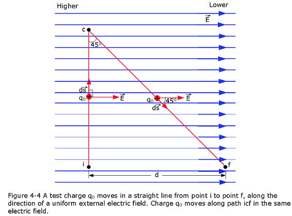
Solution:

1. Using Eq. 4-14, \[V_f-V_i = -\int_{i}^{f} \vec E.d\vec s=-E\int_{0}^{d}ds=-Ed\space (Answer)\]

2. For path ic, at all points along line ic, the displacement \(d\vec s\) of the test charge \(q_0\) is perpendicular to \(\vec E\). Thus, the angle \(\theta\) between \(\vec E\) and \(d\vec s\) is 90 , and the dot product is 0. But for path cf, the angle \(\theta = 45^\circ\) and, from Eq. 4-14, we get \[V_f-V_i = -\int_{c}^{f} \vec E.d\vec s=-E\cos45^\circ\int_{c}^{f}ds=-E\cos45^\circ\frac{d}{\cos45^\circ}=-Ed\space (Answer)\]

4.4 Potential Due to a Charged Particle:

Consider a point P at distance R from a fixed particle of positive charge q (Fig. 4-5). To use Eq. 4-11, we must evaluate the dot product

\[\begin{equation} V_f-V_i = -\int_{i}^{f} E~cos\theta~ds \tag{4.15} \end{equation}\]

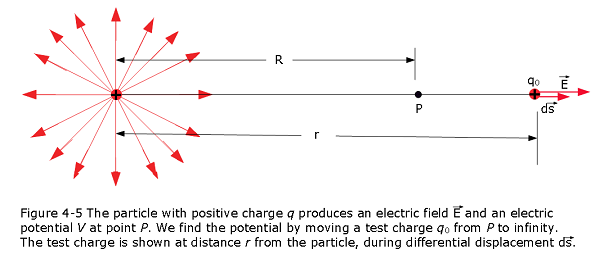
That means that in Eq. 4-13, angle \(\theta = 0\) and \(cos\theta=1\). Because the path is radial, let us write ds as dr. Then, substituting the limits i = R and \(f = \infty\), we can write Eq. 4-13 as

\[\begin{equation} V_f-V_i = -\int_{R}^{\infty} E~dr \tag{4.16} \end{equation}\]

Next, we set \(V_f=0\) (at 0) and \(V_i=V\) (at R). Then, substituting for the magnitude of the electric field at the site of the test charge, we substitute from Eq. 2-4:

\[\begin{equation} 0-V = -\frac{q}{4\pi\varepsilon_0}\int_{R}^{\infty} \frac{1}{r^2}~dr=\frac{q}{4\pi\varepsilon_0}\left[\frac{1}{r}\right]_{R}^{\infty}=-\frac{1}{4\pi\varepsilon_0}\frac{q}{R} \tag{4.17} \end{equation}\]

Thus, the potential V becomes due to a particle of charge q at any radial distance r from the particle.

\[\begin{equation} V =\frac{1}{4\pi\varepsilon_0}\frac{q}{r} \tag{4.18} \end{equation}\]

4.5 Potential Due a Group of Charged Particles:

We can find the net electric potential at a point due to a group of charged particles using the superposition principle. Using Eq. 4-18 with the plus or minus sign of the charge included, we calculate separately the potential resulting from each charge at the given point. The sum the potentials for n charges, the net potential is:

\[\begin{equation} V =\sum_{i=1}^{n}V_i=\frac{1}{4\pi\varepsilon_0}\sum_{i=1}^{n}\frac{q_i}{r_i}\space\space(n~charged~ particles). \tag{4.19} \end{equation}\]

Here \(q_i\) is the value of the ith charge and \(r_i\) is the radial distance of the given point from the ith charge.

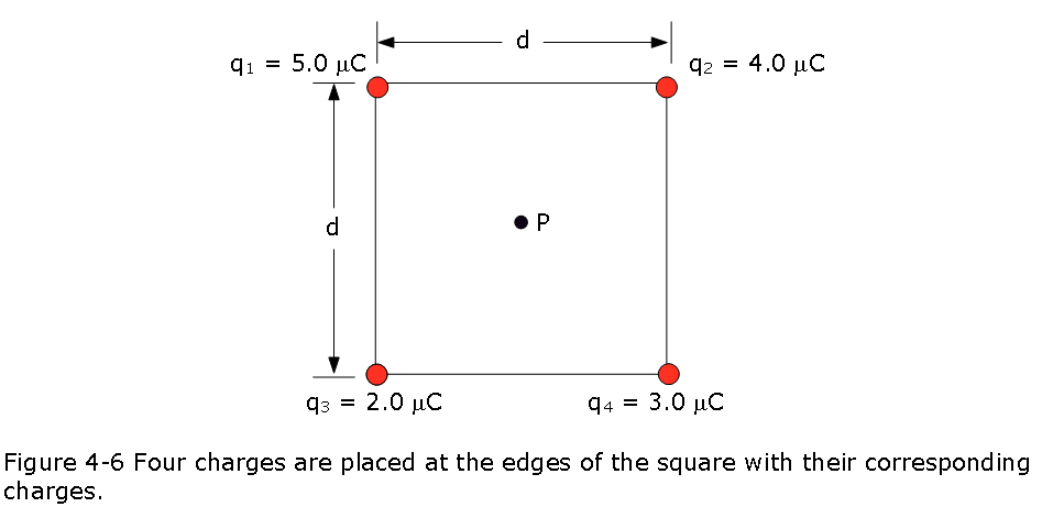
Example Problem 4.02:

What is the electric potential at point P, located at the center of the square of charged particles shown in Fig. 4-6? The distance d is 1.0 m, and the charges are

Solution:

Using Eq. 4-19, we get

\[V =\sum_{i=1}^{4}V_i=\frac{1}{4\pi\varepsilon_0}\sum_{i=1}^{n}\frac{q_i}{r_i}=\frac{1}{4\pi\varepsilon_0}\left(\frac{q_1}{r}+\frac{q_2}{r}+\frac{q_3}{r}+\frac{q_4}{r}\right)\] \[V =\left({8.99 \times 10^9}{\frac{N.m^2}{C^2}}\right)\left(\frac{5.0\mu C}{d\sqrt2}+\frac{5.0\mu C}{d\sqrt2}+\frac{5.0\mu C}{d\sqrt2}+\frac{5.0\mu C}{d\sqrt2}\right)\]

\[V =\left({8.99 \times 10^9}{\frac{N.m^2}{C^2}}\right)\left(\frac{5.0\space\mu C}{0.707\space m}+\frac{4.0\space \mu C}{0.707\space m}+\frac{2.0\space \mu C}{0.707\space m}+\frac{3.0\space\mu C}{0.707\space m}\right)=1.78\times 10^5\space (Answer)\]

4.6 Potential Due to an Electric Dipole:

Now let us apply Eq. 4-19 to an electric dipole to find the potential at an arbitrary point P in Fig. 4-7. At P, the positively charged particle (at distance \(r_{(+)}\) sets up potential \(V_{(+)}\) and the negatively charged particle (at distance \(r_{(-)}\) sets up potential \(V_{(-)}\).Then the net potential at P is given by Eq. 4-19 as

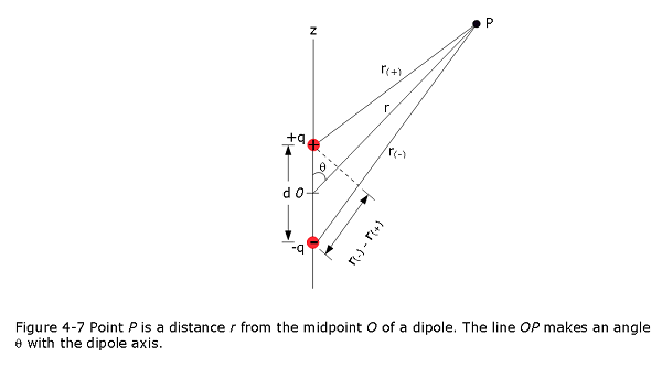
\[\begin{equation} V =\sum_{i=1}^{2}V_i=V_{(+)}-V_{(-)}=\frac{1}{4\pi\varepsilon_0}\left(\frac{q}{r_{(+)}}+\frac{-q}{r_{(-)}}\right) \tag{4.20} \end{equation}\]

\[\begin{equation} V =\frac{q}{4\pi\varepsilon_0}\frac{r_{(-)}-r_{(+)}}{r_{(-)}r_{(+)}} \tag{4.21} \end{equation}\]

As the figure suggests, the field \(\vec E\) at any point P is perpendicular to the equipotential surface through P. Also, that difference is so small that the product of the lengths is approximately \(r^2\).Thus,

\(r_{(-)}-r_{(+)}\approx dcos\theta\) \(\space\space\) \(r_{(-)}r_{(+)}\approx r^2\)

\[\begin{equation} V =\frac{q}{4\pi\varepsilon_0}\frac{d~cos\theta}{r^2} \tag{4.22} \end{equation}\]

where \(\theta\) is measured from the dipole axis as shown in Fig. 4-7. We can now write V as

\[\begin{equation} V =\frac{1}{4\pi\varepsilon_0}\frac{p~cos\theta}{r^2}\space\space(electric~dipole) \tag{4.23} \end{equation}\]

in which p = qd is the magnitude of the electric dipole moment \(\vec p\) defined in Equation 2-10.The vector \(\vec p\) is directed along the dipole axis, from the negative to the positive charge. (Thus, \(\theta\) is measured from the direction of \(\vec p\).) We use this vector to report the orientation of an electric dipole.

4.7 Potential Due to a Continuous Charge Distribution:

For a continuous charge distribution q on a uniformly charged thin rod or disk, we cannot use the summation of Eq. 4-19 to find the potential V at a point P. We have consider a differential element of charge dq, to determine the differential potential dV at P, and then integrate over the entire charge distribution. Considering the zero potential to be at infinity. Considering the differential element of charge dq as a particle, and using Eq. 4-18 we can express the potential dV at point P as:

\[\begin{equation} dV =\frac{1}{4\pi\varepsilon_0}\frac{dq}{r} \tag{4.24} \end{equation}\]

Here r is the distance between P and dq. To find the total potential V at P, we integrate to sum the potentials due to all the charge elements:

\[\begin{equation} V = \int dV =\frac{1}{4\pi\varepsilon_0}\int \frac{dq}{r} \tag{4.25} \end{equation}\]

The integral must be taken over the entire charge distribution.Note that because the electric potential is a scalar, there are no vector components to consider.

Example Problem 4.03:

Find the electric potential of a uniformly charged, nonconducting wire with linear density (coulomb/meter) and length L at a point that lies on a line that divides the wire into two equal parts.

Find the electric potential of a thin nonconducting rod of length L has a positive charge of uniform linear density \(\lambda\) (coulomb/meter). Determine the electric potential V due to the rod at point P, a perpendicular distance d from the middle of the rod as shown in Fig. 4-8.

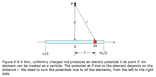
We consider a differential element dx of the rod as shown in Fig. 4-8. This (or any other) element of the rod has a differential charge of

\[\begin{equation} dq = \lambda dx \tag{4.26} \end{equation}\]

This element produces an electric potential dV at point P, which is a distance \(r = \sqrt{d^2 + x^2}\) from the element. Treating the element as a point charge, we can use Eq. 4-24 to write the potential dV as

\[\begin{equation} dV =\frac{1}{4\pi\varepsilon_0}\frac{dq}{r}=\frac{1}{4\pi\varepsilon_0}\frac{\lambda dx}{\sqrt{d^2 + x^2}} \tag{4.27} \end{equation}\]

Assuming the rod is positive and we have taken V = 0 at infinity. We now find the total potential V produced by the rod at point P by integrating Eq. 4-27 along the length of the rod, from x = -L/2 to x = +L/2, using integral in Appendix A. We find

\[\begin{equation} V =\frac{1}{4\pi\varepsilon_0}\int_{-L/2}^{+L/2}\frac{\lambda dx}{\sqrt{d^2 + x^2}}= \frac{\lambda}{4\pi\varepsilon_0}\left[ln(x+\sqrt{x^2+d^2})\right]_{-L/2}^{+L/2} \tag{4.28} \end{equation}\]

\[\begin{equation} V =\frac{\lambda}{4\pi\varepsilon_0}\left[ln\left((L/2)+\sqrt{(L/2)^2+d^2})\right)-ln\left((-L/2)+\sqrt{(-L/2)^2+d^2})\right)\right] \tag{4.29} \end{equation}\]

\[\begin{equation} V =\frac{\lambda}{4\pi\varepsilon_0}ln\left[\frac{L+\sqrt{L^2+4d^2}}{-L+\sqrt{L^2+4d^2}}\right]\space (Answer) \tag{4.30} \end{equation}\]

Example Problem 4.04:

A ring has a uniform charge density \(\lambda\), with units of coulomb per unit meter of arc. Find the electric potential at a point on the axis passing through the centre of the ring.

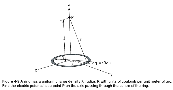
Solution:

\[\begin{equation} V =\frac{1}{4\pi\varepsilon_0}\int \frac{dq}{r}=\frac{1}{4\pi\varepsilon_0}\int_0^{2\pi}\frac{\lambda Rd \theta}{\sqrt{z^2+R^2}}=\frac{\lambda R} {4\pi\varepsilon_0\sqrt{z^2+R^2}}\int_0^{2\pi}d\theta \tag{4.31} \end{equation}\]

\[\begin{equation} V =\frac{\lambda R 2\pi} {4\pi\varepsilon_0\sqrt{z^2+R^2}}=\frac{\lambda R}{2\varepsilon_0\sqrt{z^2+R^2}}\space (Answer) \tag{4.32} \end{equation}\]

Example Problem 4.05:

A disk of radius R has a uniform charge density , with units of coulomb meter squared. Find the electric potential at any point on the axis passing through the centre of the disk.

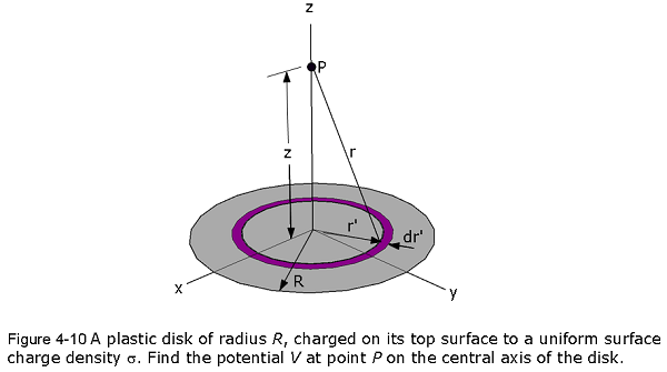
Solution:

\[\begin{equation} dV =\frac{1}{4\pi\varepsilon_0}\int \frac{dq}{r} \tag{4.33} \end{equation}\]

In Fig. 4-10, consider a differential element consisting of a flat ring of radius r’. and radial width dr’. Its charge has magnitude

\[dq = \sigma 2\pi r'dr'\] in which \(2\pi r'dr'\) is the upper surface area of the ring.

\[\begin{equation} dV =\frac{1}{4\pi\varepsilon_0}\frac{\sigma 2\pi r'dr'}{\sqrt{z^2+r'^2}} \tag{4.34} \end{equation}\]

We find the net potential at P by integrating the contributions of all the rings from r’ = 0 to r’ = R:

\[\begin{equation} V = \int dV =\frac{1}{4\pi\varepsilon_0}\int_0^R \frac{\sigma 2\pi r'dr'}{\sqrt{z^2+r'^2}}=\frac{\sigma}{2\varepsilon_0}\int_0^R \frac{r'dr'}{\sqrt{z^2+r'^2}} \tag{4.35} \end{equation}\]

\[\begin{equation} V =\frac{\sigma}{2\varepsilon_0}\int_0^R \frac{r'dr'}{\sqrt{z^2+r'^2}}=\frac{\sigma}{2\varepsilon_0}\left(\sqrt{z^2+R^2}-z\right)\space (Answer) \tag{4.36} \end{equation}\]

4.8 Calculating the Field from the Potential:

Figure 4-11 shows cross sections of a family of closely spaced equipotential surfaces, the potential difference between each pair of adjacent surfaces being dV. As the figure suggests, the field \(\vec E\) at any point P is perpendicular to the equipotential surface through P.

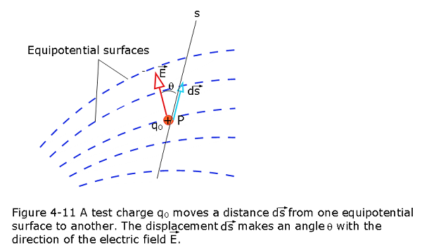
Suppose that a positive test charge \(q_0\) moves through a displacement \(d\vec s\) from one equipotential surface to the adjacent surface. From Eq. The work the electric field does on the test charge during the move is \(-q_0dV\). We also see that the work done by the electric field may also be written as the scalar product \(q_0\vec E.d\vec s\) or \(q_0E(cos\theta)ds\). Equating these two expressions for the work yields

\[-q_0dV=q_0E(cos\theta)ds\] \[E(cos\theta)=-\frac {dV}{ds}\] Since \(Ecos\theta\) is the component of \(\vec E\) in the direction of \(d\vec s\) the avbove equation becomes

\[\begin{equation} E_s = -\frac{\partial V}{\partial s} \tag{4.37} \end{equation}\]

If we take the s axis to be, in turn, the x, y, and z axes, we find that the x, y, and z components of at any point are

\[\begin{equation} E_x = -\frac{\partial V}{\partial x};\space\space E_y = -\frac{\partial V}{\partial y}; \space\space E_z = -\frac{\partial V}{\partial z} \tag{4.38} \end{equation}\]

Here we can define the “grad” or “del” vector operator, making use we can find the electric field E as the gradient of potential V. The gradient can be in Cartesian, Cylindrical or Spherical coordinate systems depending on the given problem. In Cartesian coordinate system the gradient is

\[\begin{equation} Cartesian:~\vec{\nabla}=\hat{\mathbf{i}}\frac{\partial}{\partial x}+\hat{\mathbf{j}}\frac{\partial}{\partial y}+\hat{\mathbf{k}}\frac{\partial}{\partial z}. \tag{4.39} \end{equation}\]

The electric field can be calculated as the gradient of potential as follows:

\[\begin{equation} \vec E =-\vec{\nabla}V \tag{4.40} \end{equation}\]

Problems involving cylindrical or spherical symmetry, we need to apply the del operator in the appropriate coordinates:

\[\begin{equation} Cylindrical:~\vec{\nabla}=\hat r\frac{\partial}{\partial r} +\hat \phi\frac{\partial}{\partial\phi}+\hat z\frac{\partial}{\partial z} \tag{4.41} \end{equation}\]

\[\begin{equation} Spherical:~\vec{\nabla}=\hat r\frac{\partial}{\partial r} +\hat \theta \frac{1}{r}\frac{\partial}{\partial\theta}+\hat \phi \frac{1}{r\sin\theta}\frac{\partial}{\partial \phi} \tag{4.42} \end{equation}\]

Example Problem 4.06:

Calculate the electric field of a point charge from the potential \(V = \frac{1}{4\pi\varepsilon_0}\frac{q}{r}\).

Solution:

The potential is known to be \(V = \frac{1}{4\pi\varepsilon_0}\frac{q}{r}\), which has a spherical symmetry. Therefore, we use the spherical del operator in the formula

\[\vec{\mathbf{E}}=-\vec{\nabla}V=-\left [\hat r\frac{\partial}{\partial r} +\hat \theta \frac{1}{r}\frac{\partial}{\partial\theta}+\hat \phi \frac{1}{r\sin\theta}\frac{\partial}{\partial \phi}\right]\frac{1}{4\pi\varepsilon_0}\frac{q}{r}\] \[E = -\frac{1}{4\pi\varepsilon_0}\left [\hat r\frac{\partial}{\partial r}\frac{q}{r} +\hat \theta \frac{1}{r}\frac{\partial}{\partial\theta}\frac{q}{r}+\hat \phi \frac{1}{r\sin\theta}\frac{\partial}{\partial \phi}\frac{q}{r}\right]\] \[E = -\frac{1}{4\pi\varepsilon_0}\left [\hat r\frac{\partial}{\partial r}\frac{q}{r}+0+0\right]= \frac{1}{4\pi\varepsilon_0}\left [\frac{q}{r^2}\hat r\right]\space (Answer)\]

Example Problem 4.07:

Finding the field for the potential at any point on the central axis of a uniformly charged disk.

Solution:

Using Eq. 4-36, \(V= \frac{\sigma}{2\varepsilon_0}\left(\sqrt{z^2+R^2}-z\right)\), we can get.

\[E_z = - \frac{\sigma}{2\varepsilon_0}\frac{d}{dz}\left(\sqrt{z^2+R^2}-z\right)=\frac{\sigma}{2\varepsilon_0}\left(1-\frac{z}{\sqrt{z^2+R^2}}\right)\space (Answer)\]

4.9 Electric Potential Energy of a System of Charged Particles:

Using Eq. 4-6 \((\Delta U = q(V_f - V_i))\), we can relate \((\Delta U\) to the change in potential through which we move particle 1:

\[\begin{equation} U_f-U_i = q_1(V_f - V_i) \tag{4.43} \end{equation}\]

The initial potential energy is \(U_i = 0\) because the particles are in the reference configuration.

Assuming the particle 1 is initially at distance \(r = \infty\), the potential at this location is \(V_i = 0\). When we move it to the final position at distance r, the potential at its location is

\[\begin{equation} V_f = \frac{1}{4\pi\varepsilon_0}\frac{q_2}{r} \tag{4.44} \end{equation}\]

Substituting these results into Eq. 4-39 and dropping the subscript f, we find that the final configuration has a potential energy of

\[\begin{equation} U = \frac{1}{4\pi\varepsilon_0}\frac{q_1q_2}{r}\space\space (two-particle \space system) \tag{4.45} \end{equation}\]

Example Problem 4.08:

Potential energy of a system of three charged particles Figure 4-12 shows three charged particles held in fixed positions by forces that are not shown.What is the electric potential energy U of this system of charges? Assume that d = 12 cm and that \(q_1 =+q\), \(q_2 = -4q\), and \(q_3 = +2q\), in which q = 150 nC.

Solution:

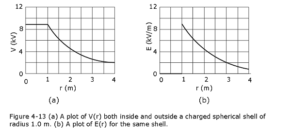
4.10 Potential of Charged Isolated Conductor:

Figure 4-13a is a plot of potential against radial distance r from the center for an isolated spherical conducting shell of 1.0 m radius, having a charge of \(1.0 \mu C\). For points outside the shell, we can calculate V(r) from Eq. 4-18 because the charge q behaves for such external points as if it were concentrated at the center of the shell.

Figure 4-13b shows the variation of electric field with radial distance for the same shell. Note that E = 0 everywhere inside the shell. The curves of Fig. 4-13b can be derived from the curve of Fig. 4-13a by differentiating with respect to r, using Eq. 4-37 (recall that the derivative of any constant is zero). The curve of Fig. 4-12a can be derived from the curves of Fig. 4-12b by integrating with respect to r, using Eq. 4-14.

4.11 Applications of Electrostatics:__

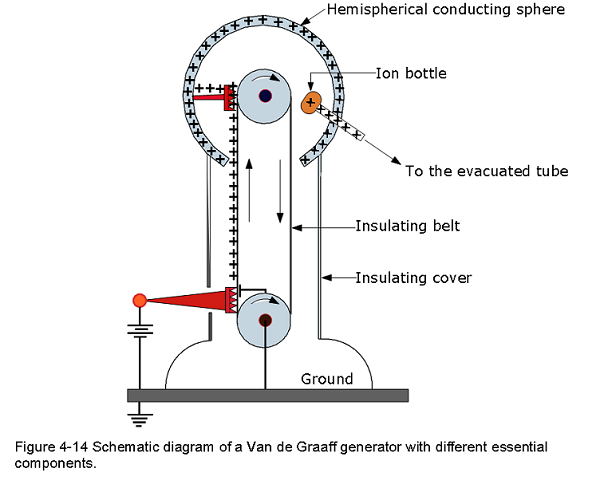
Van de Graaff: A Van de Graaff generator is an electrostatic generator which uses a moving belt to accumulate electric charge on a hollow hemispherical metal sphere which is mounted on the top of an insulated column, creating very high electric potentials. The Van de Graaff generator was developed as a particle accelerator for physics research by American physicist Robert J. Van de Graaff in 1929. The potential difference in a modern Van de Graaff generators can be as much as 5 MeV.

A Van de Graaff generator consists of an insulating belt moving over two rollers of differing material, one of which is surrounded by a hollow metal sphere. Two electrodes, in the form of comb-shaped rows of sharp metal points, are positioned one near the bottom of the lower roller to ground and the other inside the sphere, over the upper roller.

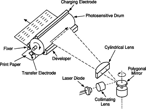
Xerography: Xerography originalyy called Xerography is a dry photocopying machine. Xerography was invented by an American physicist Chester Carlson, based significantly on contributions by a Hungarian physicist Pal Selenyi.

Solved Problems Electric Potential

1. [1] A particular 12 V car battery can send a total charge of 84 A.h (ampere-hours) through a circuit, from one terminal to the other. (a) How many coulombs of charge does this represent? (Hint: See Eq. 1-1.) (b) If this entire charge undergoes a change in electric potential of 12 V, how much energy is involved?

Solution:

1. \[q = \frac{84~C.h}{s}\frac{3600~s}{h}=3.02\times 10^5~C~(Answer)\]
2. Energy involved to undergo the charge in electric potential of 12 V is \[U = q\Delta V= (3.02\times 10^5~C)(12~V)= 3.63\times 10^6~J~(Answer)\]

2. [2] The electric potential difference between the ground and a cloud in a particular thunderstorm is \(1.2 \times 10^9\) V. In the unit electron-volts, what is the magnitude of the change in the electric potential energy of an electron that moves between the ground and the cloud?

Solution:

\[U = q\Delta V = (1.6\times 10^{-19}~C)(1.2 \times 10^9~V)\frac{1~eV}{1.6\times 10^{-19}J}=1.2~GeV~(Answer)\]

3. [6] When an electron moves from A to B along an electric field line in Fig. 4-16, the electric field does \(3.94 \times 10^{-19}\) J of work on it. What are the electric potential differences (a) \(V_B - V_A\), (b) \(V_C - V_A\), and (c) \(V_C - V_B\)?

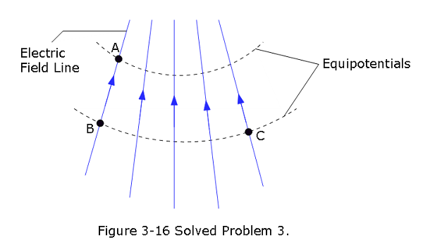
1. \[V_B-V_A = \frac{U}{q}=\frac{3.94 \times 10^{-19}~J}{1.6\times 10^{-19}~C}=2.46~V~(Answer)\]
2. \[V_C - V_A=V_B - V_A=2.46~V~(Answer)\]
3. Both C and B are in the same potential, \[V_C - V_B=0~(Answer)\]

4. [7] The electric field in a region of space has the components \(E_y = E_z = 0\) and \(E_x = (4.00~ N/C)x\). Point A is on the y axis at y 3.00 m, and point B is on the x axis at x = 4.00 m. What is the potential difference \(V_B - V_A\)?

Solution:

Using Eq. 4-13, \(V_f-V_i = -\int_{i}^{f} \vec E.d\vec s\), we get

\[V_B-V_A = -\int_{0}^{4} \vec E.d\vec s=-4.0\int_{0}^{4}xdx=-4.0\left[\frac{x^2}{2}\right]_0^4=-32~V~(Answer)\]

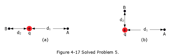
5. [14] Consider a particle with charge \(q = 1.0 \mu\) C, point A at distance \(d_1\) = 2.0 m from q, and point B at distance \(d_2\) = 1.0 m. (a) If A and B are diametrically opposite each other, as in Fig. 4-17a, what is the electric potential difference \(V_A - V_B\)? (b) What is that electric potential difference if A and B are located as in Fig. 4-17b?

Solution:

1. \[V_A-V_B = -\frac{1}{4\pi\varepsilon_0}\left[\frac{q}{d_1}-\frac{q}{d_2}\right]\] \[V_A-V_B = -\left({8.99 \times 10^9}{\frac{N.m^2}{C^2}}\right)\left[\frac{1.0 ~\mu C}{2.0~m}-\frac{1.0 ~\mu C}{1.0~m}\right]=-4.5\times 10^3~V(Answer)\]
2. Since, potential is a scalar quantity, change in configuration will not change the result.

\[V_A-V_B = -\left({8.99 \times 10^9}{\frac{N.m^2}{C^2}}\right)\left[\frac{1.0 ~\mu C}{2.0~m}-\frac{1.0 ~\mu C}{1.0~m}\right]=-4.5\times 10^3~V(Answer)\] 6. [15] A spherical drop of water carrying a charge of 30 pC has a potential of 500 V at its surface (with V = 0 at infinity). (a) What is the radius of the drop? (b) If two such drops of the same charge and radius combine to form a single spherical drop, what is the potential at the surface of the new drop?

Solution:

1. \(V = \frac{1}{4\pi\varepsilon_0}\frac{q}{r}\) \[r = \frac{1}{4\pi\varepsilon_0}\frac{q}{V}=\left({8.99 \times 10^9}{\frac{N.m^2}{C^2}}\right)\frac{30\times 10^{-12}~C}{500~V}=5.4\times 10^{-4}~m\]

2. Two drops of water increases the volume 2V, also, charge increases to 2q. The radius of the new volume is \(r' = 2^{1/3}r\)

\[V' = \frac{1}{4\pi\varepsilon_0}\frac{2q}{2^{1/3}r}=\left({8.99 \times 10^9}{\frac{N.m^2}{C^2}}\right)\frac{2\times 30\times 10^{-12}~C}{2^{1/3}5.4\times 10^{-4}~m}=793.70~V~(Answer)\]

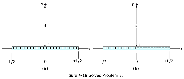
7. [23] (a) Figure 4-18a shows a nonconducting rod of length L = 6.00 cm and uniform linear charge density \(\lambda\) = +3.68 pC/m. Assume that the electric potential is defined to be V = 0 at infinity. What is V at point P at distance d = 8.00 cm along the rod’s perpendicular bisector? (b) Figure 4-18b shows an identical rod except that one half is now negatively charged. Both halves have a linear charge density of magnitude 3.68 pC/m. With V = 0 at infinity, what is V at P?

Solution:

1. Using Eq. 4-30, we can calculate V at point P at distance d = 8.00 cm along the rod’s perpendicular bisector.

\[V =\frac{\lambda}{4\pi\varepsilon_0}ln\left[\frac{L+\sqrt{L^2+4d^2}}{-L+\sqrt{L^2+4d^2}}\right]\] \[V =(3.68\times 10^{-12}~C/m)({8.99 \times 10^9}~N.m^2/C^2)ln\left[\frac{(0.06~m +\sqrt{(0.06~m)^2+4(0.08~m)^2}}{(-0.06~m +\sqrt{(0.06~m)^2+4(0.08~m)^2}}\right]\] \[V =(3.68\times 10^{-12}~C/m)({8.99 \times 10^9}~N.m^2/C^2)ln\left[ 2.08\right]=2.43\times 10^{-2}~V~(Answer)\] (b) The potential, V = 0 at P because equal and oppositie magnitudes from two sides cancel each other.

8. [26] Figure 4-19 shows a thin rod with a uniform charge density of \(2.00 \space \mu C/m\). Evaluate the electric potential at point P if d = D = L/4.00. Assume that the potential is zero at infinity.

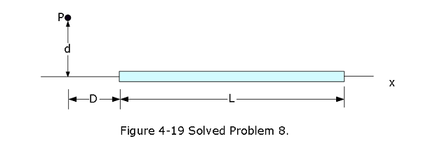
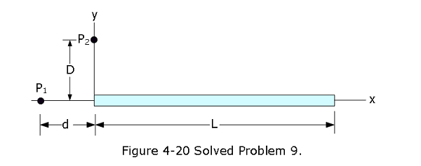
Solution: \[V = \int \frac{1}{4\pi\varepsilon_0}\frac{dq}{r}= \frac{\lambda}{4\pi\varepsilon_0}\int_D^L \frac{dx}{\sqrt {x^2+d^2}}=\frac{\lambda}{4\pi\varepsilon_0}ln\left[x+\sqrt{x^2+d^2}\right]_D^L\] \[V=\frac{\lambda}{4\pi\varepsilon_0}ln\left(\frac{L+\sqrt{L^2+d^2}}{D+\sqrt{D^2+d^2}}\right)=\frac{\lambda}{4\pi\varepsilon_0}ln\left(\frac{L+\sqrt{L^2+\frac{L^2}{16}}}{\frac{L}{4}+\sqrt{(\frac{L^2}{16}+\frac{L^2}{16})}}\right)\] \[V=\frac{\lambda}{4\pi\varepsilon_0}ln\left(\frac{L+\sqrt{L^2+\frac{L^2}{16}}}{\frac{L}{4}+\sqrt{(\frac{L^2}{16}+\frac{L^2}{16})}}\right)=\frac{\lambda}{4\pi\varepsilon_0}ln\left(\frac{L[1+\sqrt{1+\frac{1}{16}}]}{L[\frac{1}{4}+\sqrt{(\frac{1}{16}+\frac{1}{16})}]}\right)\] \[V=\frac{\lambda}{4\pi\varepsilon_0}ln\left(\frac{4+\sqrt {17}}{1+\sqrt 2}\right)=2.18\times 10^4~V~(Answer)\] 9. [28] Figure 4-20 shows a thin plastic rod of length L = 12.0 cm and uniform positive charge Q = 56.1 fC lying on an x axis. With V = 0 at infinity, find the electric potential at point \(P_1\) on the axis, at distance d = 2.50 cm from the rod.

Solution:

\[V = \int dV = \frac{1}{4\pi\varepsilon_0}\int_0^L \frac{\lambda dx}{d+x}=\frac{\lambda}{4\pi\varepsilon_0}ln(d+x)\rvert_0^L =\frac{\lambda}{4\pi\varepsilon_0}ln\left(1+\frac{L}{d}\right)\] \[V = \frac{\lambda}{4\pi\varepsilon_0}ln\left(1+\frac{L}{d}\right)=\frac{Q}{4\pi\varepsilon_0 L}ln\left(1+\frac{L}{d}\right)\] \[V =\frac{(56.1 \times 10^{-15}~C)({8.99 \times 10^9}~N.m^2/C^2)}{0.12~m}ln\left(1+\frac{0.12~m}{0.025~m}\right)=7.39\times 10^{-3}~V~(Answer)\]

10. [35] The electric potential at points in an xy plane is given by \(V = (2.0 ~V/m^2)x^2 - (3.0 ~V/m^2)y^2\). In unit-vector notation, what is the electric field at the point (3.0 m, 2.0 m)?

Solution:

Using Eq. 4-38, we find the electric field components, as follows

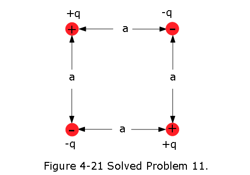
\[E_x = -\frac{\partial}{\partial x}(2.0 ~V/m^2)x^2 - (3.0 V/m^2)y^2=-2(2.0 ~V/m^2)x=-2(2.0 ~V/m^2)(3~m)=-12~V/m\] \[E_y = -\frac{\partial}{\partial y}(2.0~ V/m^2)x^2 - (3.0 ~V/m^2)y^2=2(3.0 ~V/m^2)y=2(3.0 ~V/m^2)(2~m)=12~V/m\] \[\vec E = \hat i E_x + \hat j E_y = -\hat i 12~V/m + \hat j 12~V/m~(Answer)\] 11. [43] How much work is required to set up the arrangement of Fig. 4-21 if q = 2.30 pC, a = 64.0 cm, and the particles are initially infinitely far apart and at rest?

Solution:

\[W = -\Delta U = -(U_f-U_i) = -U\], here we assumed \(U_i=0\), at infinity, and \(U = U_f\). \[W = -U=-\frac{1}{4\pi\varepsilon_0}\left[-\frac{q^2}{a}-\frac{q^2}{a}-\frac{q^2}{a}-\frac{q^2}{a}-\frac{q^2}{a\sqrt{2}}-\frac{q^2}{a\sqrt{2}}\right]\]

\[W = \frac{2q^2}{4\pi\varepsilon_0a}\left[2-\frac{1}{\sqrt{2}}\right]=\frac{2(2.30\times 10^{-12}~C)^2(8.99\times 10^9~N.m^2/C^2)}{0.640~m}\left[2-\frac{1}{\sqrt{2}}\right]\] \[W = 1.92\times 10^{-13}~J~(Answer)\] 12. [59] In Fig. 4-22, a charged particle (either an electron or a proton) is moving rightward between two parallel charged plates separated by distance d = 2.00 mm. The plate potentials are \(V_1 = -70.0\) V and \(V_2= -50.0\) V. The particle is slowing from an initial speed of 90.0 km/s at the left plate. (a) Is the particle an electron or a proton? (b) What is its speed just as it reaches plate 2?

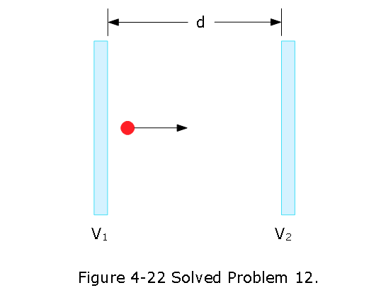
Solution: (a) According to the problem, the electric field is from right plate to the left plate. Since the particle slows down as it moves from left plate to right plate, the charged particle must be a proton.

2. The speed just as it reaches plate 2 is, \[\Delta K+\Delta V=0=K_2-K_1+U_2-U_i=\frac{1}{2}mv_2^2-\frac{1}{2}mv_1^2+qV_2-qV_1\]

\[v_2=\sqrt{\frac{2}{m}\left[\frac{1}{2}mv_1^2-qV_2+qV_1\right]}=\sqrt{\left[v_1^2-\frac{2qV_2}{m}+\frac{2qV_1}{m}\right]}\]

\[v_2=\sqrt{\left[(90.0\times 10^3 ~m/s)^2-\frac{2(1.6\times 10^{-19}~C)(-50~V)}{1.67\times 10^{-27}~kg}+\frac{2(1.6\times 10^{-19}~C)(-70~V)}{1.67\times 10^{-27}~kg}\right]}\] \[v_2=6.53\times 10^4~m/s~(Answer)\]

13. [62] Sphere 1 with radius \(R_1\) has positive charge q. Sphere 2 with radius \(2.00R_1\) is far from sphere 1 and initially uncharged. After the separated spheres are connected with a wire thin enough to retain only negligible charge, (a) is potential \(V_1\) of sphere 1 greater than, less than, or equal to potential \(V_2\) of sphere 2? What fraction of q ends up on (b) sphere 1 and (c) sphere 2? (d) What is the ratio \(\sigma_1/\sigma_2\) of the surface charge densities of the spheres?

Solution:

1. After the two spheres are connected \(V_1\) and \(V_2\) must be equal to each other.

2. Using \(V_1 = V_2\), we get

\[\frac{1}{4\pi\varepsilon_0}\frac{q_1}{R_1}=\frac{1}{4\pi\varepsilon_0}\frac{q_2}{R_2}\] Since \(q = q_1 +q_2\), and \(R_2 = 2.00R_1\), we get

\[\frac{1}{4\pi\varepsilon_0}\frac{q_1}{R_1}=\frac{1}{4\pi\varepsilon_0}\frac{q-q_1}{2.00R_1}\] Solving we get, \[\frac{q_1}{q}=\frac{1}{3}\]

and (c) \[\frac{q_2}{q}=\frac{2}{3}\]

4. \[V_1 = \frac{1}{4\pi\varepsilon_0}\frac{q_1}{R_1}=V_2 = \frac{1}{4\pi\varepsilon_0}\frac{q_2}{R_2}\] \[\frac{1}{4\pi\varepsilon_0}\frac{(\sigma_1)(4\pi R_1^2)}{R_1}= \frac{1}{4\pi\varepsilon_0}\frac{(\sigma_2)(4\pi R_2^2)}{R_2}\] \[\frac{\sigma_1}{\sigma_2}= 2~(Answer)\]

Problems Electric Potential

Section 4-1 Electric Potential

1. [3] Suppose that in a lightning flash the potential difference between a cloud and the ground is \(1.0 \times 10^9\) V and the quantity of charge transferred is 30 C. (a) What is the change in energy of that transferred charge? (b) If all the energy released could be used to accelerate a 1000 kg car from rest, what would be its final speed?

Section 4-2 Equipotential Surfaces and the Electric Field

2. [5] An infinite nonconducting sheet has a surface charge density \(\sigma = 0.10 \space \mu C/m^2\) on one side. How far apart are equipotential surfaces whose potentials differ by 50 V?

3. [10] Two uniformly charged, infinite, nonconducting planes are parallel to a yz plane and positioned at x = -50 cm and x = +50 cm. The charge densities on the planes are 50 \(nC/m^2\) and 25 \(nC/m^2\), respectively. What is the magnitude of the potential difference between the origin and the point on the x axis at x = +80 cm? (Hint: Use Gauss’ law.)

4. [11] A nonconducting sphere has radius R = 2.31 cm and uniformly distributed charge q = +3.50 fC.Take the electric potential at the sphere’s center to be \(V_0 = 0\). What is V at radial distance

1. r = 1.45 cm and (b) r = R.

Section 4-3 Potential Due to a Charged Particle

5. [12] As a space shuttle moves through the dilute ionized gas of Earth’s ionosphere, the shuttle’s potential is typically changed by -1.0 V during one revolution. Assuming the shuttle is a sphere of radius 10 m, estimate the amount of charge it collects.

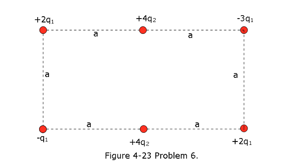
6. [16] Figure 4-23 shows a rectangular array of charged particles fixed in place, with distance a 39.0 cm and the charges shown as integer multiples of \(q_1\) = 3.40 pC and \(q_2\) = 6.00 pC. With V = 0 at infinity, what is the net electric potential at the rectangle’s center? (Hint: Thoughtful examination of the arrangement can reduce the calculation.)

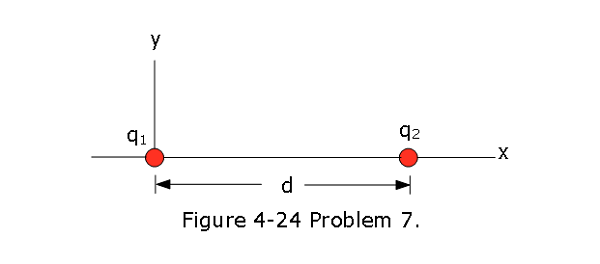
7. [19] In Fig. 4-24, particles with the charges $q_1 = +5e and \(q_2\) = -15e are fixed in place with a separation of d = 24.0 cm. With electric potential defined to be V = 0 at infinity, what are the finite (a) positive and (b) negative values of x at which the net electric potential on the x axis is zero?

Section 4-4 Potential Due to an Electric Dipole

8. [21] The ammonia molecule NH3 has a permanent electric dipole moment equal to 1.47 D, where 1 D = 1 debye unit = \(3.34 \times 10^{-30}\) C.m. Calculate the electric potential due to an ammonia molecule at a point 52.0 nm away along the axis of the dipole. (Set V = 0 at infinity.)

Section 4-5 Potential Due to a Continuous Charge Distribution

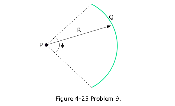
9. [24] In Fig. 4-25, a plastic rod having a uniformly distributed charge Q = -25.6 pC has been bent into a circular arc of radius R = 3.71 cm and central angle \(\phi = 120^\circ\). With V $ 0 at infinity, what is the electric potential at P, the center of curvature of the rod?

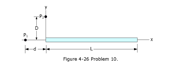
10. [28] Figure 4-26 shows a thin plastic rod of length L = 12.0 cm and uniform positive charge Q = 56.1 fC lying on an x axis. With V = 0 at infinity, find the electric potential at point \(P_1\) on the axis, at distance d = 2.50 cm from the rod.

Section 4-6 Calculating the Field from the Potential

11. [36] The electric potential V in the space between two flat parallel plates 1 and 2 is given (in volts) by \(V = 1500x^2\), where x (in meters) is the perpendicular distance from plate 1. At x = 1.3 cm, (a) what is the magnitude of the electric field and (b) is the field directed toward or away from plate 1?

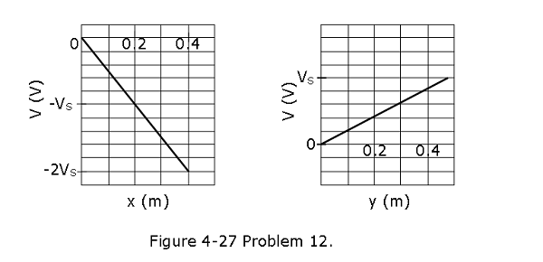
12. [39] An electron is placed in an xy plane where the electric potential depends on x and y as shown, for the coordinate axes, in Fig. 4-27 (the potential does not depend on z). The scale of the vertical axis is set by Vs 500 V. In unit-vector notation, what is the electric force on the electron?

Section 4-7 Electric Potential Energy of a System of Charged Particles

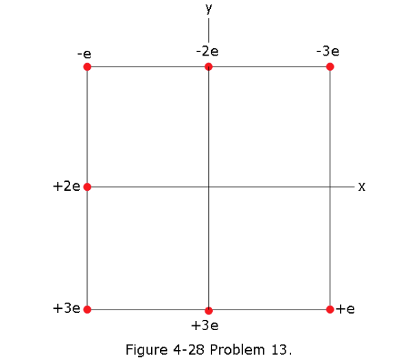
13. [44] In Fig. 4-28, seven charged particles are fixed in place to form a square with an edge length of 4.0 cm. How much work must we do to bring a particle of charge +6e initially at rest from an infinite distance to the center of the square?

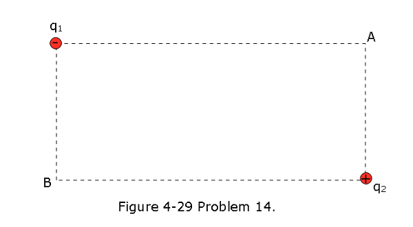
14. [51] In the rectangle of Fig. 4-29, the sides have lengths 5.0 cm and 15 cm, \(q_1 = -5.0\space \mu C\), and \(q_2 = 2.0\space \mu C\). With V = 0 at infinity, what is the electric potential at (a) corner A and

2. corner B? (c) How much work is required to move a charge \(q_3 = +3.0\space \mu C\) from B to A along a diagonal of the rectangle? (d) Does this work increase or decrease the electric potential energy of the three-charge system? Is more, less, or the same work required if \(q_3\) is moved along a path that is (e) inside the rectangle but not on a diagonal and (f) outside the rectangle?

Section 4-8 Potential of a Charged Isolated Conductor

15. [63] Two metal spheres, each of radius 3.0 cm, have a center-to-center separation of 2.0 m. Sphere 1 has charge \(1.0 \times 10^{-8}\) C; sphere 2 has charge \(-3.0 \times 10^{-8}\) C. Assume that the separation is large enough for us to say that the charge on each sphere is uniformly distributed (the spheres do not affect each other). With V = 0 at infinity, calculate (a) the potential at the point halfway between the centers and the potential on the surface of

2. sphere 1 and (c) sphere 2.

16. [64] A hollow metal sphere has a potential of +400 V with respect to ground (defined to be at V = 0) and a charge of \(5.0 \times 10^{-9}\) C. Find the electric potential at the center of the sphere.

17. [66] Two isolated, concentric, conducting spherical shells have radii \(R_1\) = 0.500 m and \(R_2\) = 1.00 m, uniform charges \(q_1 = +2.00 \mu\)C and \(q_2 = +1.00 \mu\)C, and negligible thicknesses. What is the magnitude of the electric field E at radial distance (a) r = 4.00 m, (b) r = 0.700 m, and (c) r = 0.200 m? With V = 0 at infinity, what is V at (d) r = 4.00 m, (e) r = 1.00 m, (f) r = 0.700 m, (g) r = 0.500 m, (h) r = 0.200 m, and (i) r = 0? ( j) Sketch E(r) and V(r).