Chapter 7 Circuits

Learning Objectives:

In this chapter you will basically learn:

$\bullet$ Learn for an ideal battery, how to make relationship between the emf, the current, and the power (rate of energy transfer).

$\bullet$ Learn how to draw a schematic diagram for a single-loop circuit containing a battery and three resistors.

$\bullet$ Learn the loop rule to write a loop equation that relates the potential differences of the circuit elements around a (complete) loop.

$\bullet$ Learn the resistance rule and emf rule in crossing through a resistor and emf respectively.

$\bullet$ Learn how to calculate the equivalent of series resistors and parallel resistors.

$\bullet$ Learn what is meant by grounding a circuit and that grounding a circuit does not affect the current in a circuit.

$\bullet$ Learn how to use ammeter and voltmeter with a resistor in the circuit.

$\bullet$ Learn how to write the loop equation (a differential equation) for a charging and discharging RC circuit.

$\bullet$ Learn the charging or discharging of RC circuit.

7.1 Work, Energy, and Emf:

We define the emf of the emf device in terms of this work:

\[\begin{equation} \mathcal{E}=\frac{dW}{dq}~~~(Definition~of~ \mathcal{E}) \tag{7.1} \end{equation}\]

An emf device is the work per unit charge that the device does in moving charge from its low-potential terminal to its high-potential terminal. The SI unit for emf is the joule per coulomb; in Chapter 4: Electric Potential we defined that unit as the volt.

An ideal emf device is one that has zero internal resistance. The potential difference between the terminals of an ideal emf device is equal to the emf of the device. For example, an ideal battery with an emf of 12.0 V always has a potential difference of 12.0 V between its terminals.

A real emf device, such as any real battery, has internal resistance to the internal movement of charge. We shall discuss such real batteries near the end of this module.

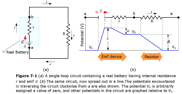
Simple Circuit with Internal Resistance: Figure 7-1a shows a real battery, with internal resistance r, wired to an external resistor of resistance R. The internal resistance of the battery is the electrical resistance of the conducting materials of the battery and thus is an unremovable feature of the battery. In Fig. 7-1a, however, the battery is drawn as if it could be separated into an ideal battery with emf # and a resistor of resistance r. The order in which the symbols for these separated parts are drawn does not matter.

If we apply the loop rule clockwise beginning at point a, the changes in potential give us

\[\begin{equation} \mathcal{E}-ir-iR=0 \tag{7.2} \end{equation}\]

Solving for the current, we find

\[\begin{equation} \mathrm{i}=\left(\frac{\mathcal{E}}{r+R}\right) \tag{7.3} \end{equation}\]

Figure 7-1b shows graphically the changes in electric potential around the circuit. (To better link Fig. 7-1b with the closed circuit in Fig. 7-1a, imagine curling the graph into a cylinder with point a at the left overlapping point a at the right.) Note how traversing the circuit is like walking around a (potential) mountain back to your starting point—you return to the starting elevation.

EXAMPLE 7.1

A given battery has a $12.00{\text -}\mathrm{V}$ emf and an internal resistance of $0.100~\Omega$. (a) Calculate its terminal voltage when connected to a $10.00{\text -}\Omega$ load. (b) What is the terminal voltage when connected to a $0.500{\text -}\Omega$ load? (c) What power does the $0.500{\text -}\Omega$ load dissipate? (d) If the internal resistance grows to $0.500~\Omega$, find the current, terminal voltage, and power dissipated by a $0.500{\text -}\Omega$ load.

Solution $(\,a)\,$ Entering the given values for the emf, load resistance, and internal resistance into the Eq. 7.1 above yields

\[i=\frac{\mathcal{E}}{R+r}=\frac{12.00~\mathrm{V}}{10.10~\Omega}=1.188~\mathrm{A}.\]

Enter the known values into the equation V_{}=-Ir to get the terminal voltage:

\[V_{\mathrm{terminal}}=\mathcal{E}-ir=12.00~\mathrm{V}-(1.188~\mathrm{A})(0.100~\Omega)=11.90~\mathrm{V}.\]

The terminal voltage here is only slightly lower than the emf, implying that the current drawn by this light load is not significant.

$(\,b)\,$ Similarly, with $R_{\mathrm{load}}=0.500~\Omega$, the current is

\[i=\frac{\mathcal{E}}{R+r}=\frac{12.00~\mathrm{V}}{0.600~\Omega}=20.00~\mathrm{A}.\]

The terminal voltage is now

\[V_{\mathrm{terminal}}=\mathcal{E}-ir=12.00~\mathrm{V}-(20.00~\mathrm{A})(0.100~\Omega)=10.00~\mathrm{V}.\]

The terminal voltage exhibits a more significant reduction compared with emf, implying 0.500~is a heavy load for this battery. A “heavy load” signifies a larger draw of current from the source but not a larger resistance.

$(\,c)\,$ The power dissipated by the $0.500{\text -}\Omega$ load can be found using the formula P=I^2R. Entering the known values gives

\[P=i^2R=(20.0~\mathrm{A})^2(0.500~\Omega)=2.00\times10^2~\mathrm{W}.\]

Note that this power can also be obtained using the expression $\frac{V^2}{R}$ or iV, where V is the terminal voltage $(10.0~\mathrm{V}$ in this case).

$(\,d)\,$ Here, the internal resistance has increased, perhaps due to the depletion of the battery, to the point where it is as great as the load resistance. As before, we first find the current by entering the known values into the expression, yielding

\[i=\frac{\mathcal{E}}{R+r}=\frac{12.00~\mathrm{V}}{1.00~\Omega}=12.0~\mathrm{A}.\]

Now the terminal voltage is

\[V_{\mathrm{terminal}}=\mathcal{E}-ir=12.00~\mathrm{V}-(12.00~\mathrm{A})(0.500~\Omega)=6.00~\mathrm{V},\]

and the power dissipated by the load is

\[P=i^2R=(12.00~\mathrm{A})^2(0.500~\Omega)=72.0\times10^2~\mathrm{W}.\]

We see that the increased internal resistance has significantly decreased the terminal voltage, current, and power delivered to a load.

Resistors Connected in Series:

The resistors in a circuit can be connected either in series and in parallel connections as can be seen in Fig. 7-2a and Fig.7-2b respectively. In a series circuit, the same current flows through in each resistor. In the parallel circuit the voltage remains the same in each resistor.

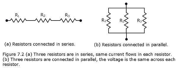
When a potential difference V is applied across resistances connected in series, the resistances have identical currents i. The sum of the potential differences across the resistances is equal to the applied potential difference V.

Figure 7-3a shows three resistances connected in series to an ideal battery with $\mathcal{E}$.

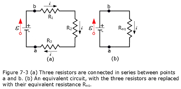
To derive an expression for $R_{eq}$ in Fig. 7-3b, we apply the loop rule to both circuits. For Fig. 7-3a, starting at a and going clockwise around the circuit, we find

\[\mathcal{E}-iR_1-iR_2-iR_3 = 0\] \[\begin{equation} i = \frac{\mathcal{E}}{R_1+R_2+R_3} \tag{7.4} \end{equation}\]

For Fig. 7-3b, with the three resistances replaced with a single equivalent resistance $R_{eq}$, we find

\[\begin{equation} i = \frac{\mathcal{E}}{R_{eq}} \tag{7.5} \end{equation}\]

Comparison of Eqs. 7-4 and 7-5 shows that

\[R_{eq}=R_1+R_2+R_3\]

Alternatively, we can derive the same result by taking the sum of the voltage applied to the circuit by the source and the potential drops across the individual resistors around a loop is equal to zero:

\[\begin{equation} \sum_{i=1}^{N}V_i=0 \tag{7.6} \end{equation}\]

This equation is often referred to as Kirchhoff’s voltage law.

\[\begin{eqnarray}\mathcal{E}-V_1-V_2-V_3&=&0,\\\Rightarrow \mathcal{E}&=&V_1+V_2+V_3\\&=&iR_1+iR_2+iR_3 \end{eqnarray}\]

\[\begin{equation} i=\frac{\mathcal{E}}{R_1+R_2+R_3}=\frac{\mathcal{E}}{R_{\mathrm{eq}}} \tag{7.7} \end{equation}\]

Since the current through each resistor is the same, the equality can be simplified to an n number of resistors that are connected in series, the equivalent resistance is

\[\begin{equation} R_{\mathrm{eq}}=R_1+R_2+R_3+\ldots+R_{N-1}+R_n=\sum_{j=1}^nR_j \tag{7.8} \end{equation}\]

EXAMPLE 7.3

A battery with a terminal voltage of $9~\mathrm{V}$ is connected to a circuit consisting of four $20{\text -}\Omega$ and one $10{\text -}\Omega$ resistors all in series (Figure 7.4). Assume the battery has negligible internal resistance. (a) Calculate the equivalent resistance of the circuit. (b) Calculate the current through each resistor. (c) Calculate the potential drop across each resistor. (d) Determine the total power dissipated by the resistors and the power supplied by the battery.

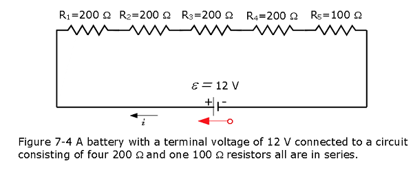
Solution $(\,a)\,$ The equivalent resistance is the algebraic sum of the resistances:

\[R_{\mathrm{eq}}=R_1+R_2+R_3+R_4+R_5=200~\Omega+200~\Omega+200~\Omega+200~\Omega+100~\Omega=900~\Omega\]

$(\,b)\,$ The current through the circuit is the same for each resistor in a series circuit and is equal to the applied voltage divided by the equivalent resistance:

\[i=\frac{V}{R_{\mathrm{eq}}}=\frac{12~\mathrm{V}}{900~\Omega}=0.01333~\mathrm{A}.\]

$(\,c)\,$ The potential drop across each resistor can be found using Ohm’s law:

\[V_1=V_2=V_3=V_4=(0.01333~\mathrm{A})200~\Omega=2.666~\mathrm{V},\]

\[V_5=(0.01333~\mathrm{A})100~\Omega=1.333~\mathrm{V},\]

\[V_1+V_2+V_3+V_4+V_5=12.0~\mathrm{V}.\]

Note that the sum of the potential drops across each resistor is equal to the voltage supplied by the battery.

$(\,d)\,$ The power dissipated by a resistor is equal to $P=i^2R$, and the power supplied by the battery is equal to P=I:

\[P_1=P_2=P_3=P_4=(0.01333~\mathrm{A})^2(200~\Omega)=0.03553778~\mathrm{W},\]

\[P_5=(0.01333~\mathrm{A})^2(100~\Omega)=0.01776889~\mathrm{W},\]

\[P_{\mathrm{dissipated}}=0.03553778~\mathrm{W}+0.03553778~\mathrm{W}+0.03553778~\mathrm{W}+0.03553778~\mathrm{W}+0.01776889~\mathrm{W}=0.1599~\mathrm{W},\]

\[P_{\mathrm{source}}=i\mathcal{E}=(0.01333~\mathrm{A})(12~\mathrm{V})=0.15996~\mathrm{W}.\]

Resistors Connected in Parallel:

Figure 7-5a shows three resistances connected in parallel to an ideal battery of $\mathcal{E}$. The term “in parallel” means that the resistances are directly wired together on one side and directly wired together on the other side, and that a potential difference V is applied across the pair of connected sides.Thus, all three resistances have the same potential difference V across them, producing a current through each. In general,

When a potential difference V is applied across resistances connected in parallel, the resistances all have that same potential difference V.

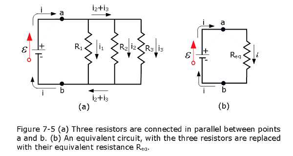
In Fig. 7-5a, the applied potential difference V is maintained by the battery. In Fig. 7-45b, the three parallel resistances have been replaced with an equivalent resistance $R_{eq}$.

Resistances connected in parallel can be replaced with an equivalent resistance $R_{eq}$ that has the same potential difference V and the same total current i as the actual resistances.

To derive an expression for $R_{eq}$ in Fig. 7-5b, we first write the current in each actual resistance in Fig. 7-5a as

\[\begin{eqnarray} i_1= \frac{V}{R_1},~i_2= \frac{V}{R_2},~and~i_3= \frac{V}{R_3} \end{eqnarray}\]

where V is the potential difference between a and b. If we apply the junction rule at point a in Fig. 7-5a and then substitute these values, we find

\[\begin{equation} i = i_1+i_2+i_3 = V\left(\frac{1}{R_1}+\frac{1}{R_2}+ \frac{1}{R_3}\right) \tag{7.9} \end{equation}\]

If we replaced the parallel combination with the equivalent resistance $R_{eq}$ (Fig. 7-5b), we would have

\[\begin{equation} i = \frac{V}{R_{eq}} \tag{7.10} \end{equation}\]

Comparing Eqs. 7-9 and 7-10 leads to

\[\begin{equation} \frac{1}{R_{eq}} = \left(\frac{1}{R_1}+\frac{1}{R_2}+ \frac{1}{R_3}\right) \tag{7.11} \end{equation}\]

Extending this result to the case of n resistances, we have (n resistances in parallel).

\[\begin{equation} \frac{1}{R_{eq}}=\sum_{j=1}^n\frac{1}{R_j} \tag{7.12} \end{equation}\]

Table 7-1 Series and Parallel Resistors and Capacitors.

	Series		Parallel
Equivalent resistance	$R_{eq} = \sum_{j=1}^{n}R_j~$Eq. 7.8		$\frac{1}{R_{eq}} = \sum_{j=1}^{n}\frac{1}{R_j}~$Eq. 7.12
Equivalent capacitor	$\frac{1}{C_{eq}} = \sum_{j=1}^{n}\frac{1}{C_j}~$Eq. 5.18		$C_{eq} = \sum_{j=1}^{n}C_j~$Eq. 5.17

Example 7.4

Three resistors $R_1=1.00~\Omega$, $R_2=2.00~\Omega$, and $R_3=2.00~\Omega$ are connected in parallel. The parallel connection is attached to a V=3.00~ voltage source. (a) What is the equivalent resistance? (b) Find the current supplied by the source to the parallel circuit. (c) Calculate the currents in each resistor and show that these add together to equal the current output of the source. (d) Calculate the power dissipated by each resistor. (e) Find the power output of the source and show that it equals the total power dissipated by the resistors.

Solution: $(\,a)\,$ The total resistance for a parallel combination of resistors is found using Equation 6.2.2. Entering known values gives

\[R_{\mathrm{eq}}=\left(\frac{1}{R_1}+\frac{1}{R_2}+\frac{1}{R_3}\right)^{-1}=\left(\frac{1}{1.00~\Omega}+\frac{1}{2.00~\Omega}+\frac{1}{2.00~\Omega}\right)^{-1}=0.50~\Omega\]

The total resistance with the correct number of significant digits is $R_{\mathrm{eq}}=0.50~\Omega$. As predicted, $R_{\mathrm{eq}}$ is less than the smallest individual resistance.

$(\,b)\,$ The total current can be found from Ohm’s law, substituting $R_{\mathrm{eq}}$ for the total resistance. This gives

\[i=\frac{V}{R_{\mathrm{eq}}}=\frac{3.00~\mathrm{V}}{0.50~\Omega}=6.00~\mathrm{A}.\]

Current i for each device is much larger than for the same devices connected in series (see the previous example). A circuit with parallel connections has a smaller total resistance than the resistors connected in series.

$(\,c)\,$ The individual currents are easily calculated from Ohm’s law, since each resistor gets the full voltage. Thus,

\[i_1=\frac{V}{R_1}=\frac{3.00~\mathrm{V}}{1.00~\Omega}=3.00~\mathrm{A}.\]

Similarly,

\[i_2=\frac{V}{R_2}=\frac{3.00~\mathrm{V}}{2.00~\Omega}=1.50~\mathrm{A}.\]

and

\[i_3=\frac{V}{R_3}=\frac{3.00~\mathrm{V}}{2.00~\Omega}=1.50~\mathrm{A}.\]

The total current is the sum of the individual currents:

\[i_1+i_2+i_3=6.00~\mathrm{A}.\]

$(\,d)\,$ The power dissipated by each resistor can be found using any of the equations relating power to current, voltage, and resistance, since all three are known. Let us use P=V^2/R, since each resistor gets full voltage. Thus,

\[P_1=\frac{V^2}{R_1}=\frac{(3.00~\mathrm{V})^2}{1.00~\Omega}=9.00~\mathrm{W}.\]

Similarly,

\[P_2=\frac{V^2}{R_2}=\frac{(3.00~\mathrm{V})^2}{2.00~\Omega}=4.50~\mathrm{W}.\]

and

\[P_3=\frac{V^2}{R_3}=\frac{(3.00~\mathrm{V})^2}{2.00~\Omega}=4.50~\mathrm{W}.\]

$(\,e)\,$ The total power can also be calculated in several ways. Choosing P=iV and entering the total current yields

\[P=iV=(6.00~\mathrm{A})(3.00~\mathrm{V})=18.00~\mathrm{W}.\]

7.2 Potential Difference Between Two Points, Multiloop Circuits:

Combinations of series and parallel can be reduced to a single equivalent resistance using the technique illustrated in Example 7.5.

Example 7.5

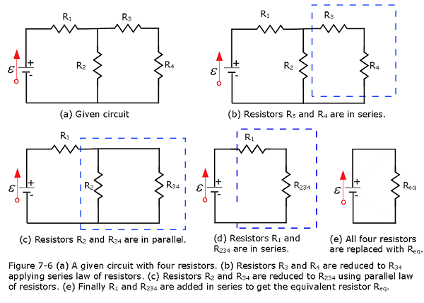
In the Example 7.5, a given circuit with four resistors $R_1 = 7~\Omega$, $R_2 = 10~\Omega$, $R_3 = 6~\Omega$, $R_4 = 7~\Omega$ are connected either in series or in parallel with an emf device of $\mathcal{E} = 24~V$. Find (a) the equivalent resistance $R_{eq}$ in the circuit, (b) voltage drops in each of the resistors, (c) power dissipates in each of the resistors, and (d) the power supplied by the emf source.

Solution:

$(\,a)\,$ The resistors $R_3$ and $R_4$ are in series and can be added as follows:

\[R_{34}=R_3+R_4=6~\Omega+4~\Omega=10~\Omega.\]

The circuit now reduces to three resistors, shown in Figure 7.6(c). Redrawing, we now see that resistors $R_2$ and $R_{34}$ constitute a parallel circuit. Those two resistors can be reduced to an equivalent resistance:

\[R_{234}=\left(\frac{1}{R_2}+\frac{1}{R_{34}}\right)^{-1}=\left(\frac{1}{10~\Omega}+\frac{1}{10~\Omega}\right)^{-1}=5~\Omega.\]

Now two resistors $R_1$, and $R_{234}$ are in series as shown in Figure 7.6 (d). These two resistors can be combined in series to an equivalent resistance:

\[R_{\mathrm{eq}}=R_{1234}=R_1+R_{234}=7~\Omega+5~\Omega=12~\Omega.\]

$(\,b)\,$ The total current provided by the voltage source is $i=\frac{V}{R_{\mathrm{eq}}}=\frac{24~\mathrm{V}}{12~\Omega}=2~\mathrm{A}$. This current runs through resistor $R_1$ and is designated as $i_1$. The potential drop across $R_1$ can be found using Ohm’s law:

\[V_1=i_1R_1=(2~\mathrm{A})(7~\Omega)=14~\mathrm{V}.\]

Looking at Figure 7.6(c), this leaves $24~\mathrm{V}-14~\mathrm{V}=10~\mathrm{V}$ to be dropped across the parallel combination of $R_2$ and $R_{34}$. The current through $R_2$ can be found using Ohm’s law:

\[i_2=\frac{V_2}{R_2}=\frac{10~\mathrm{V}}{10~\Omega}=1~\mathrm{A}.\]

The resistors $R_3$ and $R_4$ are in series so the currents $i_3$ and $i_4$ are equal to

$i_3=i_4=i-i_2=2~\mathrm{A}-1~\mathrm{A}=1~\mathrm{A}.$

Using Ohm’s law, we can find the potential drop across the last two resistors. The potential drops are $V_3=i_3R_3=6~\mathrm{V}$ and $V_4=i_4R_4=4~\mathrm{V}$. The final analysis is to look at the power supplied by the voltage source and the power dissipated by the resistors.

$(\,c)\,$ \[\begin{eqnarray} P_1&=&i_1^2R_1=(2~\mathrm{A})^2(7~\Omega)=28~\mathrm{W},\\P_2&=&i_2^2R_2=(1~\mathrm{A})^2(10~\Omega)=10~\mathrm{W},\\P_3&=&i_3^2R_3=(1~\mathrm{A})^2(6~\Omega)=6~\mathrm{W},\\P_4&=&i_4^2R_4=(1~\mathrm{A})^2(4~\Omega)=4~\mathrm{W},\\P_{\mathrm{dissipated}}&=&P_1+P_2+P_3+P_4=48~\mathrm{W}. \end{eqnarray}\]

$(\,d)\,$ The total energy is constant in any process. Therefore, the power supplied by the voltage source is

$P_s=iV=(2~\mathrm{A})(24~\mathrm{V})=48~\mathrm{W}$. Analyzing the power supplied to the circuit and the power dissipated by the resistors is a good check for the validity of the analysis; they should be equal.

Example 7.6 Figure 7.7 shows resistors wired in a combination of series and parallel. We can consider $R_1$ to be the resistance of wires leading to $R_2$ and $R_3$ (a) Find the equivalent resistance of the circuit. (b) What is the potential drop $V_1$ across resistor $R_1$? (c) Find the current $i_2$ through resistor $R_2$. (d) What power is dissipated by $R_2$?

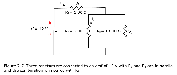
$(\,a)\,$ To find the equivalent resistance of the circuit, notice that the parallel connection of $R_2$ and $R_3$ is in series with $R_1$, so the equivalent resistance is

\[R_{\mathrm{eq}}=R_1+\left(\frac{1}{R_2}+\frac{1}{R_3}\right)^{-1}=1.00~\Omega+\left(\frac{1}{6.00~\Omega}+\frac{1}{13.00~\Omega}\right)^{-1}=5.10~\Omega.\]

The total resistance of this combination is intermediate between the pure series and pure parallel values $(20.0~\Omega$ and $0.804~\Omega$, respectively).

$(\,b)\,$ The current through $R_1$ is equal to the current supplied by the battery:

\[i_1=i=\frac{V}{R_{\mathrm{eq}}}=\frac{12.0~\mathrm{V}}{5.10~\Omega}=2.35~\mathrm{A}.\]

The voltage across $R_1$ is

\[V_1=i_1R_1=(2.35~\mathrm{A})(1~\Omega)=2.35~\mathrm{V}.\]

The voltage applied to $R_2$ and $R_3$ is less than the voltage supplied by the battery by an amount $V_1$. When wire resistance is large, it can significantly affect the operation of the devices represented by $R_2$ and $R_3$.

$(\,c)\,$ To find the current through $R_2$, we must first find the voltage applied to it. The voltage across the two resistors in parallel is the same:

\[V_2=V_3=V-V_1=12.0~\mathrm{V}-2.35~\mathrm{V}=9.65~\mathrm{V}.\]

Now we can find the current $i_2$ through resistance $R_2$ using Ohm’s law:

\[i_2=\frac{V_2}{R_2}=\frac{9.65~\mathrm{V}}{6.00~\Omega}=1.61~\mathrm{A}.\]

The current is less than the $2.00~\mathrm{A}$ that flowed through $R_2$ when it was connected in parallel to the battery in the previous parallel circuit example.

$(\,d)\,$ The power dissipated by $R_2$ is given by

\[P_2=i_2^2R_2=(1.61~\mathrm{A})^2(6.00~\Omega)=15.5~\mathrm{W}.\]

7.3 Kirchhoff’s Voltage and Current Rules

Kirchhoff’s current rule is the sum of all currents entering a junction must equal the sum of all currents leaving the junction:

\[\begin{equation} \sum i_{in}=\sum i_{out} \end{equation}\]

Kirchhoff’s voltage second rule is the algebraic sum of changes in potential around any closed circuit path (loop) must be zero:

\[\begin{equation} \sum V=0 \end{equation}\]

7.4 The Ammeter and the Voltmeter:

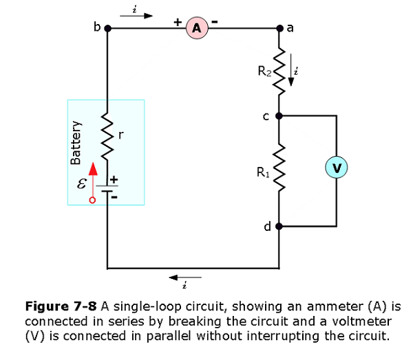
An instrument that we use to measure the electric currents is called an ammeter. To measure the current (i) in a wire, we insert the ammeter (A) in series by breaking or cutting the wire so that the current can be passed through the meter as shown in Fig. 7-8. The accuracy of measuring the electric current in an electric circuit depends on the internal resistance of the ammeter itself $R_A$ must be very much smaller than other resistances in the circuit.

An electrical instrument that is used to measure potential differences is called a voltmeter. To measure the voltage or the potential difference between any two points in the circuit, the voltmeter terminals are connected between those points without breaking or cutting the wire as shown in Fig. 7-8. In Fig. 7-8 the voltmeter V is set up to measure the voltage across $R_1$ with the condition that the resistance $R_V$ of a voltmeter must be very much larger than the total resistances of any circuit element across which the voltmeter is connected.

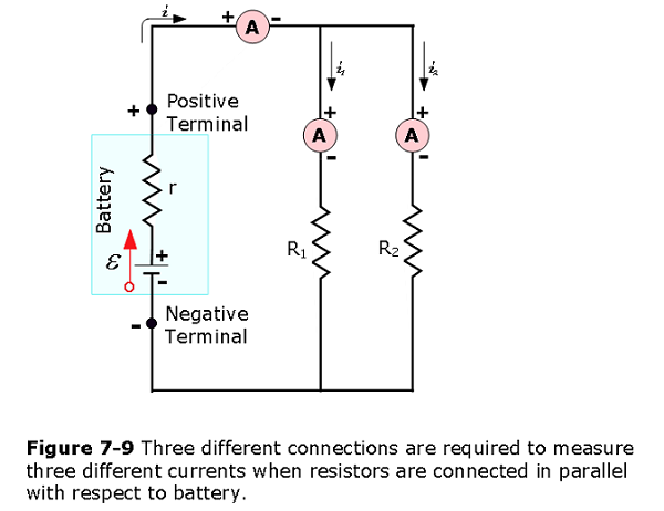
One single ammeter is used to measure the current through two resistors connected in series to a battery, since the same current passes through the two resistors are same in series. But in Figure 7-9 when the two resistors are connected in parallel with a battery, three separate ammeters are required to measure the individual currents from the battery that pass through each and every individual resistor.

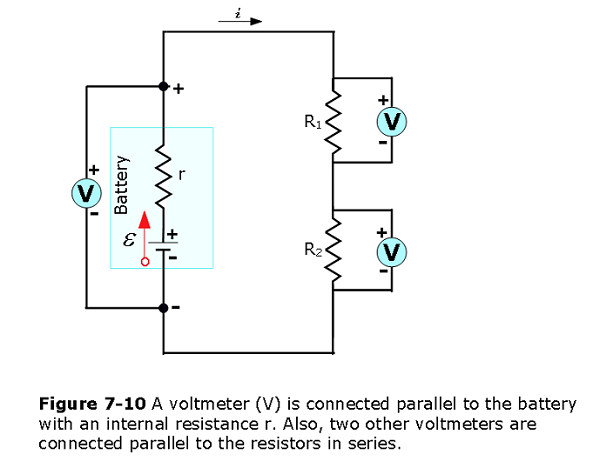
In Fig. 7-10 a voltmeter (V) is placed in parallel with the voltage source or either of the resistors. Note that terminal voltage is measured between the positive terminal and the negative terminal of the battery or voltage source. It is not possible to connect a voltmeter directly across the emf without including the internal resistance r of the battery.

7.5 RC Circuits:

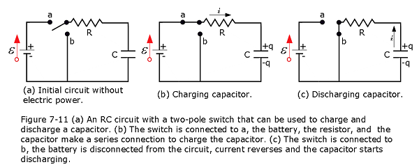
So far we discussed circuits without the time varying components such as capacitor. We will consider an RC circuit to find the time-varying currents and its effect in charging and discharging a capacitor. The capacitor of capacitance C in Fig. 7-11 is initially uncharged. To charge it, we close the switch S on point a. This completes an RC series circuit consisting of the capacitor, an ideal battery of emf $\mathcal{E}$, and a resistance R.

Using Kirchhoff’s voltage rule in the charging of the capacitor, the sum of the voltage drops across the capacitor ($V_C=\frac{q}{C}$) and voltage drop across the resistor ($V_R=iR$) is zero. Furthermore, using $i=\frac{dq}{dt}$ and traversing through the circuit as shown in Fig. 7-11, we come up with the following equation.

\[\begin{equation} \mathcal{E}= R\frac{dq}{dt}+\frac{q}{C}~~~(charging~equation) \tag{7.13} \end{equation}\]

Rearranging Eqn. 7-13 and letting $u=\mathcal{E}C-q$ and $du=-dq$ and integrating both sides of the equation we come up with the

\[-\int_0^q\frac{du}{u}=\frac{1}{RC}\int_0^tdt\]

\[\ln\left(\frac{\mathcal{E}C-q}{\mathcal{E}C}\right)=-\frac{1}{RC}t,\]

\[\frac{\mathcal{E}C-q}{\mathcal{E}C}=e^{-t/RC}.\]

Simplifying results in an equation for the charge on the charging capacitor as a function of time:

\[\begin{equation} q(t)=C\mathcal{E}\left(1-e^{-\frac{t}{RC}}\right)~~~(charging ~a~ capacitor) \tag{7.14} \end{equation}\]

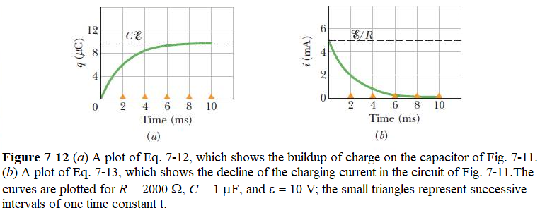
In analyzing Eq. 7-14, we can find that at t = 0 the term $e^{-\frac{t}{RC}}$ becomes unity and as a result the equation gives q = 0. Also as t goes to infinity, the term $e^{-\frac{t}{RC}}$ goes to zero and the equation gives the full (equilibrium) charge on the capacitor,$C\mathcal{E}$. A plot of q(t) for the charging process is given in Fig. 7-12a.

The derivative of q(t) in Eqn. 7-14 is the current i(t) charging the capacitor:

\[\begin{equation} i(t)=\frac{dq}{dt}=\frac{\mathcal{E}}{R}e^{-\frac{t}{RC}}~~~(charging ~a~ capacitor) \tag{7.15} \end{equation}\]

At time $t=0.00~\mathrm{s}$, the current through the resistor is $i_0=\frac{\mathcal{E}}{R}$. As time approaches infinity, the current approaches zero.

As the charge on the capacitor increases, the current decreases, as does the voltage difference across the resistor $V_R(t)=(I_0R)e^{-t/RC}=\mathcal{E}e^{-t/RC}$. The voltage difference across the capacitor increases as

\[\begin{equation} V_C(t)=\frac{q}{C}=\mathcal{E}\left(1-e^{-t/RC}\right)~~~(charging ~a~ capacitor) \tag{7.16} \end{equation}\]

This tells us that $V_C= 0$ at $t = 0$ and that $V_C = \mathcal{E}$ when the capacitor becomes fully charged as $t\to\infty$.

Capacitive Time Constant: The product RC that appears in Eqs. 7-14, 7-15, and 7-16 has the dimensions of time (both because the argument of an exponential must be dimensionless and because, in fact, $1.0 \Omega \times 1.0 F = 1.0 s)$. The product RC is called the capacitive time constant of the circuit and is represented with the symbol t:

\[\begin{equation} \tau = RC ~~~(capacitive~time~constant) \tag{7.17} \end{equation}\]

From Eq. 7-14, we can now see that at time $t=\tau = RC$, the charge on the initially uncharged capacitor of Fig. 7-11 has increased from zero to

\[\begin{equation} q(t=RC)=C\mathcal{E}\left(1-e^{-1}\right)=0.63C\mathcal{E} \tag{7.18} \end{equation}\]

Charge builds across the capacotor in one time constant $t=\tau = RC$ from zero to 63% of its maximum value $C\mathcal{E}$. In Fig. 7-12, the small triangles along the time axes mark successive intervals of one time constant during the charging of the capacitor.

Discharging a Capacitor The differential equation describing q(t) in Eq. 7-13 can be modified to see the effect of discharging of a capacitor without a battery in the circuit as follows:

\[\begin{equation} R\frac{dq}{dt}+\frac{q}{C}=0 ~~~(discharging~equation). \tag{7.19} \end{equation}\]

The solution to this differential equation is

\[\begin{equation} q(t)=q_0 e^{-t/\tau}~~~(discharging~a~capacitor) \tag{7.20} \end{equation}\]

where $q_0 = CV_0$ is the initial charge on the capacitor.

Differentiating Eq. 7-20 gives us the current i(t):

\[\begin{equation} i(t)=\frac{dq}{dt}= -\left(\frac{q_0}{RC}\right)e^{-t/RC}~~~(discharging~a~capacitor) \tag{7.21} \end{equation}\]

Eq. 7-21 tells us that the current also decreases exponentially with time, at a rate set by t. The initial current $i_0$ is equal to $q_0/RC$. Note that you can find $i_0$ by simply applying the loop rule to the circuit at $t = 0$; just then the capacitor’s initial potential $V_0$ is connected across the resistance R, so the current must be $i_0 = V_0/R= \frac{q_0}{RC}$. The minus sign in Eq. 7-21 can be ignored, it means that the capacitor’s charge q is decreasing.

Example 7.6 One application of an RC circuit is the flashing light, as shown in Fig. 7-13. The flashing light consists of a voltage source, a resistor, a capacitor, and a fluorescent lamp. The fluorescent lamp acts like an open circuit (infinite resistance) until the potential difference across the fluorescent lamp reaches a specific voltage. At that voltage, the fluorescent lamp acts like a short circuit (zero resistance), and the capacitor discharges through the fluorescent lamp and produces light. In the flashing light, the voltage source charges the capacitor until the voltage across the capacitor is $80~\mathrm{V}$. When this happens, the fluorescent lamp breaks down and allows the capacitor to discharge through the lamp, producing a bright flash. After the capacitor fully discharges through the fluorescent lamp, it begins to charge again, and the process repeats. Assuming that the time it takes the capacitor to discharge is negligible, what is the time interval between the consecutive flashes?

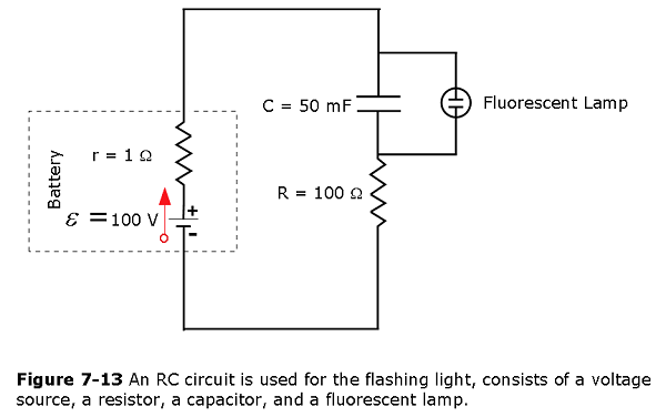
Solution: The flashing lamp flashes when the voltage across the capacitor reaches 80 V. The RC time constant is equal to $\tau=(R+r)C=(101~\Omega)(50\times10^{-3}~\mathrm{F})=5.05~\mathrm{s}$. We can solve the voltage equation for the time it takes the capacitor to reach $80~\mathrm{V}$:

\[\begin{eqnarray} V_C(t)&=&\mathcal{E}\left(1-e^{-t/\tau}\right),\\e^{-t/\tau}&=&1-\frac{V_C(t)}{\mathcal{E}},\\\ln\left(e^{-t/\tau}\right)&=&\ln\left(1-\frac{V_C(t)}{\mathcal{E}}\right),\\t&=&-\tau\,\ln\left(1-\frac{V_C(t)}{\mathcal{E}}\right)=-5.05~\mathrm{s}\cdot\ln\left(1-\frac{80~\mathrm{V}}{100~\mathrm{V}}\right)=8.13~\mathrm{s}. \end{eqnarray}\]

EXAMPLE 7.7 A flashing light circuit as given above can also be used to control the car windshield wipers. The flashing light consists of a $10.00{\text -}\mathrm{mF}$ capacitor and a $10.00{\text -}\mathrm{k}\Omega$ variable resistor known as a potentiometer. A knob connected to the variable resistor allows the resistance to be adjusted from $0.00~\Omega$ to $10.00~\Omega$. The output of the capacitor is used to control a voltage-controlled switch. The switch is normally open, but when the output voltage reaches $10.00~\mathrm{V}$, the switch closes, energizing an electric motor and discharging the capacitor. The motor causes the windshield wipers to sweep once across the windshield and the capacitor begins to charge again. To what resistance should the potentiometer be adjusted for the period of the wiper blades be 10.00 seconds?

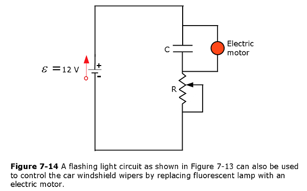
Solution The output voltage will be $10.00~\mathrm{V}$ and the voltage of the battery is $12.00~\mathrm{V}$. The capacitance is given as $10.00~\mathrm{mF}$. Solving for the resistance yields

\[\begin{eqnarray} V_{\mathrm{out}}(t)&=&V\left(1-e^{-t/\tau}\right)\\e^{-t/RC}&=&1-\frac{V_{\mathrm{out}}(t)}{V},\\\ln\left(e^{-t/RC}\right)&=&\ln\left(1-\frac{V_{\mathrm{out}}(t)}{V}\right),\\-\frac{t}{RC}&=&\ln\left(1-\frac{V_{\mathrm{out}}(t)}{V}\right),\\R&=&\frac{-t}{C\ln\left(1-\frac{V_{\mathrm{out}}(t)}{V}\right)}=\frac{-10.00~\mathrm{s}}{(10\times10^{-3}~\mathrm{F})\ln\left(1-\frac{10~\mathrm{V}}{12~\mathrm{V}}\right)}\\&=&558.11~\Omega \end{eqnarray}\]

Solved Problems Circuits

[1] In Fig. 7-15, the ideal batteries have emfs $\mathcal{E}_1$ = 12 V and $\mathcal{E}_2$ = 6.0 V. What are (a) the current, the dissipation rate in (b) resistor 1 (4.0~$\Omega$) and (c) resistor 2 (8.0 ~$\Omega$), and the energy transfer rate in (d) battery 1 and (e) battery 2? Is energy being supplied or absorbed by (f) battery 1 and (g) battery 2?

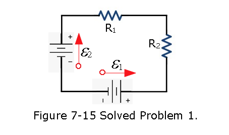
Solution: Given $\mathcal{E_1}$=12 V and $\mathcal{E}_2$ = 6.0 V, traversing through the circuit counter clockwise we get,

\[\mathcal{E_1}-\mathcal{E_2}-iR_2-iR_1=0\] $(\,a)\,$ The current dissipation rate \[i = \frac{\mathcal{E_1}-\mathcal{E_2}}{R_1+R_2}=\frac{12~V-6~V}{4~\Omega+8~\Omega}=0.5~A~(Answer)\]

$(\,b)\,$ $P_1 = i^2R_1=(0.5~A)^2(4~\Omega)=1~W~(Answer)$ $(\,c)\,$ $P_2 = i^2R_2=(0.5~A)^2(8~\Omega)=2~W~(Answer)$ $(\,d)\,$ $P_1=i\mathcal{E_1}=(0.5~A)(12~V)=6~W~(Answer)$ $(\,e)\,$ $P_2=i\mathcal{E_2}=(0.5~A)(6~V)=3~W~(Answer)$ $(\,f)\,$ Battery 1 supplies energy to the circuit and is discharging. $(\,g)\,$ Battery 2 absorbs energy and is charging.

[7] A wire of resistance 5.0 $\Omega$ is connected to a battery whose emf $\mathcal{E}$ is 2.0 V and whose internal resistance is 1.0 $\Omega$. In 2.0 min, how much energy is (a) transferred from chemical form in the battery, (b) dissipated as thermal energy in the wire, and (c) dissipated as thermal energy in the battery?

Solution:

$(\,a)\,$ \[E_1 = Pt = \mathcal{E}it=\frac{\mathcal{E^2}}{R+r}t=\frac{(2.0~V)^2(2~min)(60~s/1~min)}{1.0~\Omega+5.0~\Omega}=80~J~(Answer)\]

$(\,b)\,$ Energy dissipated in the wire: $E_2 = i^2Rt=\left(\frac{\mathcal{E}}{R+r}\right)^2Rt$

\[E_2=\left(\frac{2~V}{1~\Omega+5~\Omega}\right)^2(5~\Omega)(2~min)(60~s/1~min)=67~J~(Answer)\] $(\,c)\,$ Energy dissipated as thermal energy in the battery: \[E = E_1-E_2=(80-67)~J=13~J~(Answer)\]

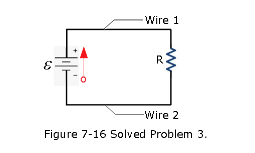
[12] Figure 7-16 shows a resistor of resistance R = 6.00 $\Omega$ connected to an ideal battery of emf $\mathcal{E}$ = 12.0 V by means of two copper wires. Each wire has length 20.0 cm and radius 1.00 mm. In dealing with such circuits in this chapter, we generally neglect the potential differences along the wires and the transfer of energy to thermal energy in them. Check the validity of this neglect for the circuit of Fig. 7-16. What is the potential difference across (a) the resistor and (b) each of the two sections of wire? At what rate is energy lost to thermal energy in (c) the resistor and (d) each section of wire?

Solution:

To find the voltage drop across the resistor, R, we use $V = iR_{tot}$, where $R_{tot}$ is the total resistance in the circuit.

To find the resistance of the wire we can use Eq. 6.6, $R_{wire} = \frac{\rho L}{A}=\frac{\rho L}{\pi r^2}$ and getting the resistivity data for copper from Table 6.1, we get

\[R_{wire} = \frac{\rho L}{\pi r^2}= \frac{(1.69\times 10^{-8}~\Omega.m)(0.20~m)}{\pi (1.0\times 10^{-3}~m)^2}=0.001075887~\Omega.\] Total resistance in the circuit is

\[R_{tot}=R + 2R_{wire}=6.00 ~\Omega+2(0.001075887~\Omega)=6.0022~\Omega\] The current in the circuit $i = \frac{V}{R_{eq}} = \frac{12~V}{6.0022~\Omega}=1.9992~A$.

The voltage drop across the resistor, R, becomes

\[V_R = iR = (1.9992~A)(6.00 ~\Omega) = 11.995~V~(Answer)\] (b) Voltage drop in each section of the wire is

\[V_{wire} = iR_{wire}= (1.9992~A)(0.001075887~\Omega)=0.0022~V~(Answer)\] (c) Power dissipated in the resistor

\[P_R= i^2R = (1.9992~A)^2(6.00 ~\Omega)=23.98~W~(Answer)\] (d) Power dissipated in each section of the wire

\[P_{wire}= i^2R_{wire} = (1.9992~A)^2(0.001075887~\Omega)=0.0043~W~(Answer)\]

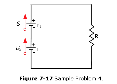
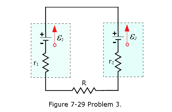
[17] In Fig. 7-17, battery 1 has emf $\mathcal{E}_1$ = 12.0 V and internal resistance $r_1$ = 0.016 $\Omega$ and battery 2 has emf $\mathcal{E}_2$ = 12.0 V and internal resistance $r_2$ = 0.012 $\Omega$. The batteries are connected in series with an external resistance R. (a) What R value makes the terminal-to-terminal potential difference of one of the batteries zero? (b) Which battery is that?

Solution:

Traversing through the circuit, we get

\[\mathcal{E_2}-ir_2+\mathcal{E_1}-ir_1-iR = 0\] Solving for current, \[i = \frac{\mathcal{E_2}+\mathcal{E_1}}{r_1+r_2+R}\]

To make the terminal-to-terminal potential difference of one of the batteries zero, with the given condition that battery 1 has the higher internal resistance, and it will meet the condition of zero terminal voltage that is $\mathcal{E_1 = ir_1}$ or $i = \frac{\mathcal{E_1}}{r_1}$. Solving algebra, we get

\[R=\frac{r_1\mathcal{E_2}-r_2\mathcal{E_1}}{\mathcal{E_1}}\] Given $\mathcal{E_1}=\mathcal{E_2}=12~V$, gives

\[R = r_1-r_2 = (0.016-0.012)\Omega=0.04~\Omega~(Answer)\] (b) Instead of choosing the battery 1, if we consider battery 2, we get \[R = r_2-r_1 = (0.016-0.012)\Omega=-0.04~\Omega\]. But negative resistance is unacceptable. Therefore, battery 1 is the answer.

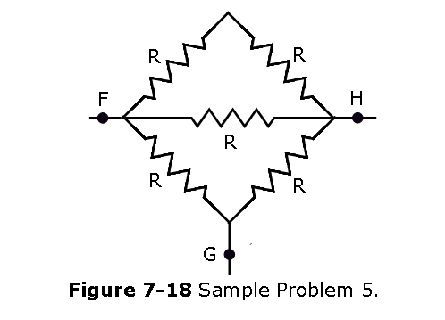
[22] Figure 7-18 shows five 5.00 $\Omega$ resistors. Find the equivalent resistance between points (a) F and H and (b) F and G. (Hint: For each pair of points, imagine that a battery is connected across the pair.)

Solution:

Equivalent resistance between points F and H is: \[\frac{1}{R_{FH}} = \frac{1}{2R} + \frac{1}{R} + \frac{1}{2R}=\frac{2}{R}\] \[R_{FH} = \frac{R}{2}=\frac{5~\Omega}{2}=2.5~\Omega~(Answer)\]
Equivalent resistance between points F and G is:

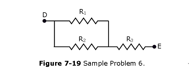
\[\frac{1}{2R}+\frac{1}{R}=\frac{3}{2R}\] \[R+\frac{2R}{3}=\frac{5R}{3}\] \[\frac{1}{R_{FG}}= \frac{1}{R}+\frac{3}{5R} = \frac{8}{5R}\] \[R_{FG} = \frac{5R}{8}= \frac{5(5~\Omega)}{8}=3.125~\Omega~(Answer)\] 6. [24] In Fig. 7-19, $R_1$ = $R_2$ = 4.00 $\Omega$ and $R_3$ = 2.50 $\Omega$. Find the equivalent resistance between points D and E. (Hint: Imagine that a battery is connected across those points.)

Solution:

\[R_{DE} = \left(\frac{1}{R_1}+ \frac{1}{R_2}\right)^{-1}+R_3=\frac{R_1R_2+R_3(R_1+R_2)}{(R_1+R_2)}\] \[R_{DE} = \frac{R_1R_2+R_3(R_1+R_2)}{(R_1+R_2)}=\frac{(4~\Omega)(4~\Omega)+2.50~\Omega(4~\Omega+4~\Omega)}{(4~\Omega+4~\Omega)}=4.5~\Omega~(Answer)\]

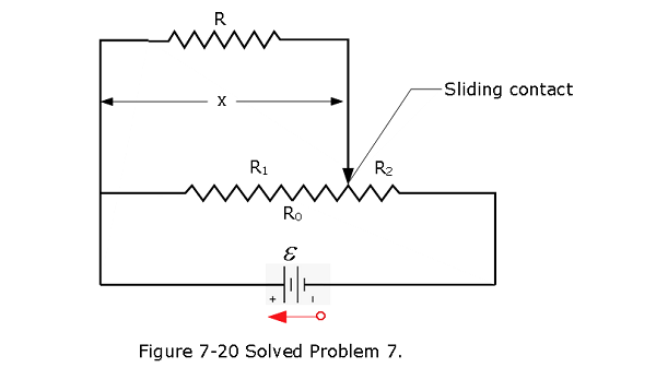
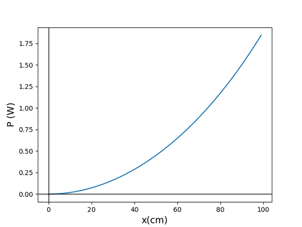
[26] Figure 7-20 shows a battery connected across a uniform resistor $R_0$. A sliding contact can move across the resistor from x = 0 at the left to x = 10 cm at the right. Moving the contact changes how much resistance is to the left of the contact and how much is to the right. Find the rate at which energy is dissipated in resistor R as a function of x. Plot the function for $\mathcal{E}$ = 50 V, R = 2000 $\Omega$, and $R_0$ = 100 $\Omega$.

Solution:

\[R_2 = (1-\frac{x}{L})R_0\] \[R_{eq} = R_2 + R_P=(1-\frac{x}{L})R_0+\frac{RR_1}{R+R_1}\] Since $R_P$ is connected in series with $R_2$ $I_P = I_2$ ; $\frac{V_P}{R_P}=\frac{V_2}{R_2}$; $\mathcal{E} = V_P+V_2$; $V_2 = \mathcal{E}-V_P; V_P = \frac{\mathcal{E}R_P}{R_2+R_P}$

$R_1$ and $R$ are in parallel, therefore, \[V_R = V_P = \frac{R_P\mathcal{E}}{R_2+R_P}=\frac{RR_1\mathcal{E}}{R_1R_2+RR_0}\] \[P_R = \frac{V_R^2}{R} = \frac{100R(\frac{\mathcal{E}x}{R_0})^2}{\left(\frac{100R}{R_0}+10x-x^2\right)^2}\] The python plot of $P_R$ versus x is shown below:

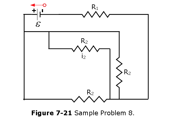
[29] In Fig. 7-21, $R_1 = 6.00 ~\Omega$, $R_2 = 18.0 ~\Omega$, and the ideal battery has emf $\mathcal{E}$ = 12.0 V. What are the (a) size and (b) direction (left or right) of current $i_1$? (c) How much energy is dissipated by all four resistors in 1.00 min?

Solution:

The equivalent resistance in the circuit is \[R_{eq} = \frac{R_2}{3}+R_1 = \frac{18~\Omega}{3} + 6~\Omega= 12 ~\Omega\] Total current passes through the circuit is \[i = \frac{\mathcal{E}}{R_{eq}}= \frac{12~V}{12~\Omega}= 1~A\] Voltage drop across the resistor, $R_1$, is \[V_1 = iR_1 = (1 ~A)(6~\Omega) = 6~V\] \[V_1+V_2 = \mathcal{E}; V_2 =\mathcal{E}-V_1=(12-6)~V=6~V\] \[i_1=\frac{V_2}{R_2}=\frac{6~V}{18~\Omega}=\frac{1}{3}~A~(Answer)\]
The direction of the is rightward.
Power dissipated $P=i^2R_{eq}=(1~A)^2(12~\Omega)=12~W$ Energy is dissipated by all four resistors in 1.00 min, is \[E = Pt=(12~W)(60~s)= 720~J~(Answer)\]

[32] Both batteries in Fig. 7-22a are ideal. Emf $\mathcal{E}_1$ of battery 1 has a fixed value, but emf $\mathcal{E}_2$ of battery 2 can be varied between 1.0 V and 10 V. The plots in Fig. 7-22b give the currents through the two batteries as a function of $\mathcal{E}_2$. The vertical scale is set by is $i_s$ 0.20 A. You must decide which plot corresponds to which battery, but for both plots, a negative current occurs when the direction of the current through the battery is opposite the direction of that battery’s emf. What are (a) emf $\mathcal{E}_1$, (b) resistance $R_1$, and (c) resistance $R_2$?

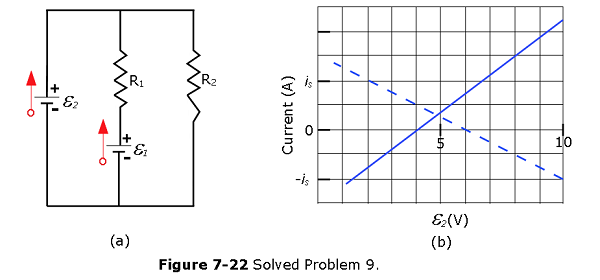
Solution: In order to solve the problem, we need to understand the plots of Figure 7-22 and identify the solid line and dashed line and their corresponding batteries and currents. The plot indicates that the current versus $\mathcal{E_2}$, so the y-axis current must be $i_2$ and the dashed line is the current $i_1$ for the battery $\mathcal{E_1}$.

Since the battery $\mathcal{E_1}$ is fixed in value, we can have the following two cases happen:

Case-I: $\mathcal{E_1}\gt \mathcal{E_2}$, we have the following equations

\[\mathcal{E_1}-i_1R_1-\mathcal{E_2}=0\] and

\[\mathcal{E_1}-i_1R_1-i_3R_2=0\] Considering $\mathcal{E_2} = 4~V$, we get $i_2 = 0$ and $i_1 = 0.1~A$, we get, and in this case current flows through the right loop:

\[\mathcal{E_1}-0.1R_1-0.1R_2=0\] \[\mathcal{E_1}=0.1(R_1+R_2)\] Case-II: $\mathcal{E_1}\lt \mathcal{E_2}$, we have the following equations

\[\mathcal{E_2}-i_1R_1-\mathcal{E_1}=0\] \[\mathcal{E_2}-i_3R_2=0\] For $\mathcal{E_2}=6~V$, the corresponding $i_1 = 0$ from the plot. Therefore, we get \[\mathcal{E_1}=6~V\]

Now for $\mathcal{E_2}=6~V$,the corresponding $i_2 = 0.3~A$ and $i_1 = 0.1~A$ from the plot. Since $i_2 = i_1+i_3$, we get $i_3 = 0.2~A$ and \[8-0.1R_1-6=0\] and \[R_1 = 20~\Omega\] and \[R_2 = ~40~\Omega\]

[36] In Fig. 7-23, $\mathcal{E}_1$ = 6V,$\mathcal{E}_2$ = 12 V, $R_1$ = 100 $\Omega$, $R_2$ = 200 $\Omega$ and $R_3$ = 300 $\Omega$. One point of the circuit is grounded (V = 0). What are the (a) size and (b) direction (up or down) of the current through resistance 1, the (c) size and (d) direction (left or right) of the current through resistance 2, and the (e) size and (f) direction of the current through resistance 3? (g) What is the electric potential at point A?

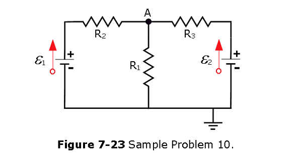
Solution: Using loop rules of circuit, we get the following equations,

\[\mathcal{E_1}-i_2R_2-(i_2+i_3)R_1=0\] \[\mathcal{E_2}-i_3R_3-(i_2+i_3)R_1=0\] Plug in the given values of the problem, we get \[6~V-200i_2-100(i_2+i_3)=0\] \[12~V-300i_3-100(i_2+i_3)=0\] Solving the above two equations we get, \[i_2 = 0.0109~A\] and \[i_3 = 0.0273~A\], hence

\[i_1 = i_2+I3 = 0.0109+0.0273 = 0.0382~A~(Answer)\]
The direction of $i_1$ is downward
\[i_2 = 0.0109~A\]
The direction of $i_2$ is rightward
\[i_3 = 0.0273~A\]
The direction of $i_3$ is leftward

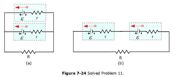
[40] Two identical batteries of emf $\mathcal{E}$ = 12.0 V and internal resistance r = 0.200 $\Omega$ are to be connected to an external resistance R, either in parallel (Fig. 7-24a) or in series (Fig. 7-24b). If R = 2.00r, what is the current i in the external resistance in the (a) parallel and (b) series arrangements? (c) For which arrangement is i greater? If R = r/2.00, what is i in the external resistance in the (d) parallel arrangement and (e) series arrangement? (f) For which arrangement is i greater now?

Solution:

Applying junction rule of current, $i = i_1 + i_2$ Applying loop rule in the upper loop, we get \[\mathcal{E}-i_1r-\mathcal{E}+i_2r=0\] Applying loop rule in the lower loop, we get

\[iR-\mathcal{E}+i_1r=0\] Solving the three equations we get current in the parallel connection

\[i = \frac{2\mathcal{E}}{r+2R}=\frac{2(\times 12~V)}{0.2~\Omega+2(2\times0.2~\Omega)}=24~A\] (b) For $R = 2.00r$, in series \[2\mathcal{E}-2ir-iR = 0\] \[i = \frac{2\mathcal{E}}{2r+R}=\frac{2(\times 12~V)}{2(0.2~\Omega)+(2\times0.2~\Omega)}=30~A\]

$R \gt r$, series current is more than parallel current.
If $R = \frac{r}{2.00}$, for parallel connection,

\[i = \frac{2\mathcal{E}}{r+2R}=\frac{2(\times 12~V)}{0.2~\Omega+2\frac{(0.2~\Omega)}{2}}=60~A\]

\[i = \frac{2\mathcal{E}}{2r+R}=\frac{2(\times 12~V)}{2(0.2~\Omega)+\frac{0.2~\Omega}{2}}=48~A\]
$R \lt r$, parallel current is more than series current.

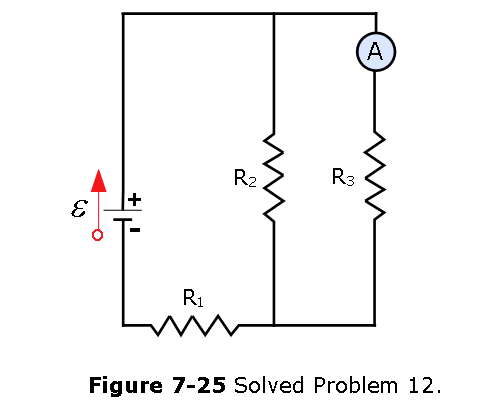
[49] (a) In Fig. 7-25, what current does the ammeter read if $\mathcal{E}$ = 5.0 V (ideal battery), $R_1$ = 2.0 $\Omega$, $R_2$ = 4.0 $\Omega$, and $R_3$ = 6.0 $\Omega$? (b) The ammeter and battery are now interchanged. Show that the ammeter reading is unchanged.

Solution:

The current through the resistor $R_1$, \[i_1 = \frac{\mathcal{E}}{R_{eq}}=\frac{\mathcal{E}}{R_1+\frac{R_2R_3}{R_2+R_3}}=\frac{5~V}{\left(2+\frac{4\times 6}{4+6}\right)\Omega}=1.14~A\]

Current through ammeter is \[i_3 =\frac{V_3}{R_3}=\frac{\mathcal{E}-i_1R_1}{R_3}=\frac{5~V-(1.14~A\times 2\Omega)}{6~\Omega}=0.45~A\] (b) The current through the resistor $R_3$, \[i_3 = \frac{\mathcal{E}}{R_{eq}}=\frac{\mathcal{E}}{R_3+\frac{R_1R_2}{R_1+R_3}}=\frac{5~V}{\left(6+\frac{2\times 4}{2+4}\right)\Omega}=0.682~A\]

Current through ammeter is \[i_1 =\frac{\mathcal{E}-i_3R_3}{R_1}=\frac{5~V-(0.682~A\times 6\Omega)}{2~\Omega}=0.45~A\] Therefore, interchanging the ammemeter and battery doesn’t change the value of current.

[54] When the lights of a car are switched on, an ammeter in series with them reads 10.0 A and a voltmeter connected across them reads 12.0 V (Fig. 7-26). When the electric starting motor is turned on, the ammeter reading drops to 8.00 A and the lights dim somewhat. If the internal resistance of the battery is 0.0500 $\Omega$ and that of the ammeter is negligible, what are (a) the emf of the battery and (b) the current through the starting motor when the lights are on?

Solution:

Emf of the battery is \[\mathcal{E} = v +ir = 12~V+(10.0~A)(0.0500~\Omega)=12.5~V~(Answer) \]
The current through the starting motor when the lights are on is \[\mathcal{E}=i_AR_{light}+(i_m+8.00~A)r\], or

\[i_m = \frac{\mathcal{E}-i_AR_{light}}{r}-8~A= \frac{12.5~V-(8~A)(12~V/10~A)}{0.050~\Omega}-8~A=50~A~(Answer)\]

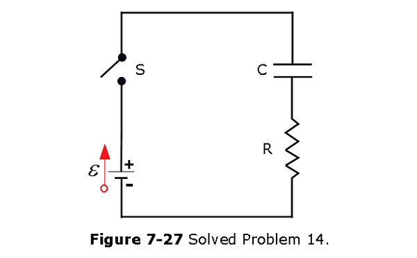
[57] Switch S in Fig. 7-27 is closed at time t = 0, to begin charging an initially uncharged capacitor of capacitance C = 15.0 $\mu$F through a resistor of resistance R = 20.0 $\Omega$. At what time is the potential across the capacitor equal to that across the resistor?

Solution:

\[q = C\mathcal{E}\left(1-e^{-t/RC}\right)\] \[i = \frac{dq}{dt} = \frac{\mathcal{E}}{R}\left(e^{-t/RC}\right)\] Given condition, $V_R = V_C$ \[\mathcal{E}e^{-t/RC}=\mathcal{E}(1-e^{-t/RC})\] \[t = RCln2 = 0.208~ms~(Answer)\] 15. [60] A capacitor with initial charge $q_0$ is discharged through a resistor. What multiple of the time constant t gives the time the capacitor takes to lose (a) the first one-third of its charge and (b) two-thirds of its charge?

Solution:

During discharging of a capacitor, \[q=q_0e^{-t/\tau}; t = \tau ln{(q_0/q)}\] \[t_{1/3} = \tau ln\frac{q_0}{2q_0/3}=0.41\tau~(Answer)\]
\[t_{2/3} = \tau ln\frac{q_0}{q_0/3}=1.1\tau~(Answer)\]

Problems Circuits

Section 7-1 Single-Loop Circuits

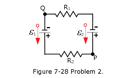
[2] In Fig. 7-28, the ideal batteries have emfs $\mathcal{E}_1$ = 150 V and $\mathcal{E}_2$ = 50 V and the resistances are $R_1 = 3.0 ~\Omega$ and $R_2 = 2.0 ~\Omega$. If the potential at P is 100 V, what is it at Q?

[6] A standard flashlight battery can deliver about 2.0 W.h of energy before it runs down. (a) If a battery costs US$0.80, what is the cost of operating a 100 W lamp for 8.0 h using batteries?

What is the cost if energy is provided at the rate of US$0.06 per kilowatt-hour?

[10] (a) In Fig. 27-28, what value must R have if the current in the circuit is to be 1.0 mA? Take $\mathcal{E}_1$ = 2.0 V, $\mathcal{E}_2$ = 3.0 V, and $r_1 = r_2 = 3.0 ~\Omega$. (b) What is the rate at which thermal energy appears in R?

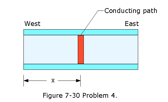
[13] A 10-km-long underground cable extends east to west and consists of two parallel wires, each of which has resistance 13 $\Omega$/km. An electrical short develops at distance x from the west end when a conducting path of resistance R connects the wires (Fig. 7-30). The resistance of the wires and the short is then 100 $\Omega$ when measured from the east end and 200 $\Omega$ when measured from the west end. What are (a) x and (b) R?

Section 7-2 Multiloop Circuits

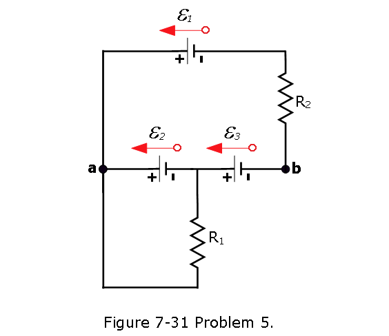
[23] In Fig. 7-31, $R_1$ = 100 $\Omega$, $R_2$ = 50 $\Omega$, and the ideal batteries have emfs $\mathcal{E}_1$ = 6.0 V, $\mathcal{E}_2$ = 5.0 V, and $\mathcal{E}_3$ = 4.0 V. Find (a) the current in resistor 1, (b) the current in resistor 2, and (c) the potential difference between points a and b.

[25] Nine copper wires of length l and diameter d are connected in parallel to form a single composite conductor of resistance R. What must be the diameter D of a single copper wire of length l if it is to have the same resistance?
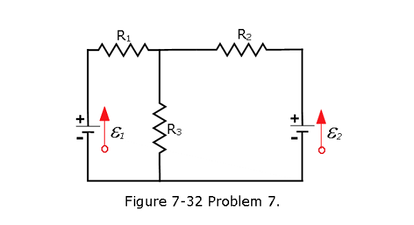
[30] In Fig. 7-32, the ideal batteries have emfs $\mathcal{E}_1$ = 10.0 V and $\mathcal{E}_2$ = $\mathcal{E}_10.005$ V, and the resistances are each 4.00 $\Omega$. What is the current in (a) resistance 2 and (b) resistance 3?

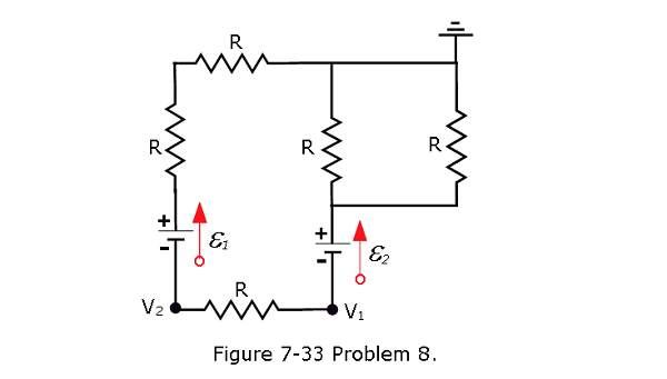
[31] In Fig. 7-33, the ideal batteries have emfs $\mathcal{E}_1$ = 5.0 V and $\mathcal{E}_2$=2.0~V, the resistances are each 2.0 $\Omega$, and the potential is defined to be zero at the grounded point of the circuit.What are potentials (a) $V_1$ and (b) $V_2$ at the indicated points?

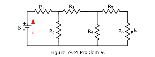
[33] In Fig. 7-34, the current in resistance 6 is $i_6$ = 1.40 A and the resistances are $R_1 = R_2 = R_3 = 2.00 \Omega$, $R_4 = 16.0 \Omega$, $R_5 = 8.00 \Omega$, and $R_6 = 4.00 \Omega$. What is the emf of the ideal battery?

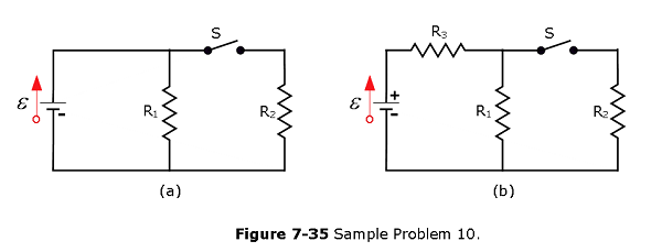
[34] The resistances in Figs. 7-35a and b are all 6.0 $\Omega$, and the batteries are ideal 12 V batteries. (a) When switch S in Fig. 27-45a is closed, what is the change in the electric potential $V_1$ across resistor 1, or does $V_1$ remain the same? (b) When switch S in Fig. 7-35b is closed, what is the change in $V_1$ across resistor 1, or does $V_1$ remain the same?

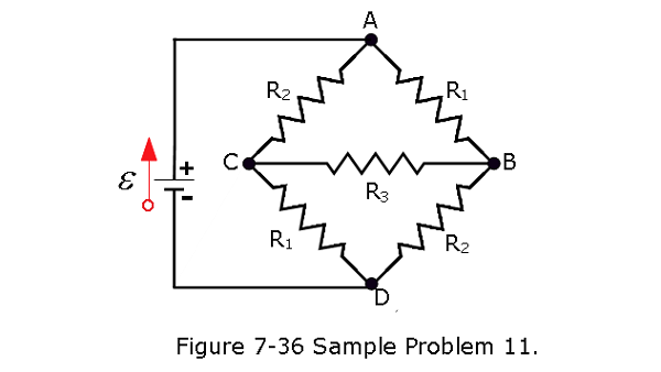
[35] In Fig. 7-36, $\mathcal{E}$ = 12.0 V, $R_1$ = 2000 ~$\Omega$, $R_2$ = 3000 ~$\Omega$, and $R_3$ = 4000 ~$\Omega$. What are the potential differences (a) $V_A - V_B$, (b) $V_B - V_C$, (c) $V_C - V_D$, and (d) $V_A - V_C$?

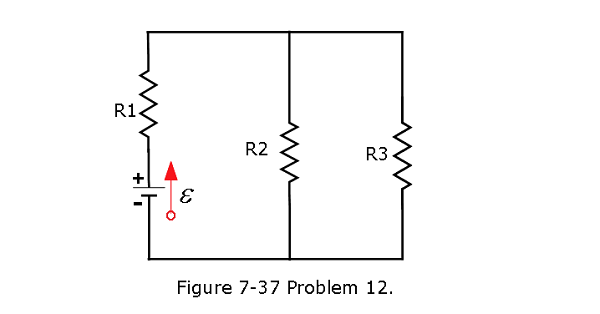
[37] In Fig. 7-37, the resistances are $R_1$ = 2.00 $\Omega$, $R_2$ = 5.00 $\Omega$, and the battery is ideal. What value of $R_3$ maximizes the dissipation rate in resistance 3?

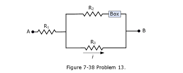
[38] Figure 7-38 shows a section of a circuit. The resistances are $R_1$ = 2.0 $\Omega$,$R_2$ = 4.0 $\Omega$, and $R_3$ = 6.0 $\Omega$, and the indicated current is i = 6.0 A. The electric potential difference between points A and B that connect the section to the rest of the circuit is $V_A - V_B$ = 78 V. (a) Is the device represented by “Box” absorbing or providing energy to the circuit, and (b) at what rate?

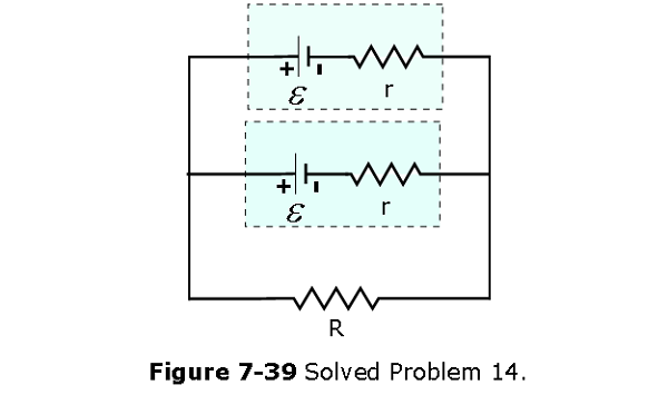
[39] In Fig. 7-39, two batteries with an emf V and an internal resistance r = 0.300 $\Omega$ are connected in parallel across a resistance R. (a) For what value of R is the dissipation rate in the resistor a maximum? (b)What is that maximum?

[41] In Fig. 7-32, $\mathcal{E}_1$ = 3.00 V, $\mathcal{E}_1$ = 1.00 V, $R_1$ = 4.00 $\Omega$, $R_2$ = 2.00 $\Omega$, $R_3$ = 5.00 $\Omega$, and both batteries are ideal. What is the rate at which energy is dissipated in (a) $R_1$, (b) $R_2$, and (c) $R_3$? What is the power of (d) battery 1 and (e) battery 2?

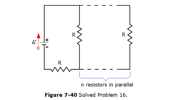
[42] In Fig. 7-40, an array of n parallel resistors is connected in series to a resistor and an ideal battery. All the resistors have the same resistance. If an identical resistor were added in parallel to the parallel array, the current through the battery would change by 1.25%. What is the value of n?

[43] You are given a number of 10 $\Omega$ resistors, each capable of dissipating only 1.0 W without being destroyed. What is the minimum number of such resistors that you need to combine in series or in parallel to make a 10 $\Omega$ resistance that is capable of dissipating at least 5.0 W?
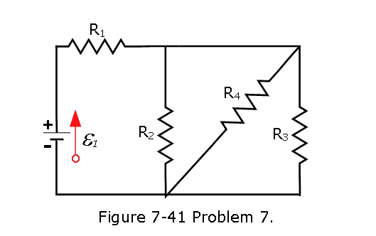
[44] In Fig. 7-41, $R_1$ = 100 $\Omega$, $R_2 = R3$ = 50.0 $\Omega$, $R_4$ = 75.0 $\Omega$, and the ideal battery has emf $\mathcal{E}$ = 6.00 V. (a) What is the equivalent resistance? What is i in (b) resistance 1, (c) resistance 2, (d) resistance 3, and (e) resistance 4?

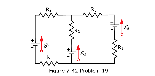
[45] In Fig. 7-42, the resistances are $R_1$ = 1.0 $\Omega$ and $R_2$ = 2.0 $\Omega$, and the ideal batteries have emfs $\mathcal{E}_1$ = 2.0 V and $\mathcal{E}_2$ = $\mathcal{E}_3$ = 4.0 V. What are the (a) size and (b) direction (up or down) of the current in battery 1, the (c) size and (d) direction of the current in battery 2, and the (e) size and (f) direction of the current in battery 3? (g) What is the potential difference $V_a - V_b$?

Section 27-3 The Ammeter and the Voltmeter

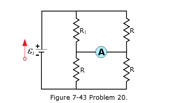
[50] In Fig. 7-43, $R_1$ = 2.00R, the ammeter resistance is zero, and the battery is ideal. What multiple of $\frac{\mathcal{E}}{R}$ gives the current in the ammeter?

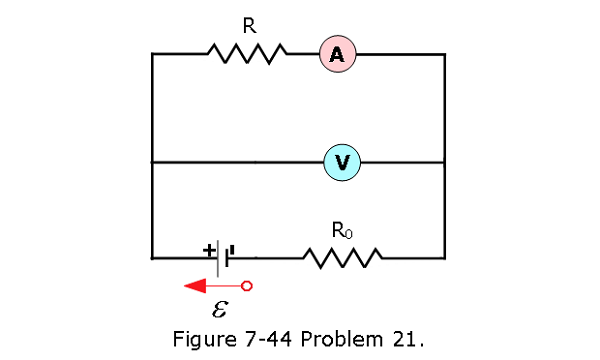
[51] In Fig. 7-44, a voltmeter of resistance $R_V$ = 300 $\Omega$ and an ammeter of resistance $R_A$ = 3.00 $\Omega$ are being used to measure a resistance R in a circuit that also contains a resistance $R_0$ = 100 $\Omega$ and an ideal battery with an emf of $\mathcal{E}$ = 12.0 V. Resistance R is given by R = V/i, where V is the potential across R and i is the ammeter reading. The voltmeter reading is V’, which is V plus the potential difference across the ammeter. Thus, the ratio of the two meter readings is not R but only an apparent resistance R’ = V’/i. If R = 85.0 $\Omega$, what are (a) the ammeter reading, (b) the voltmeter reading, and (c) R’? (d) If $R_A$ is decreased, does the difference between R’ and R increase, decrease, or remain the same?

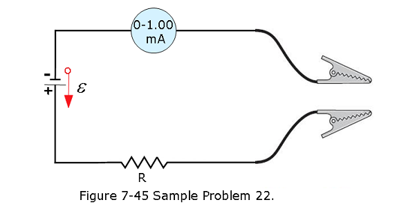
[52] A simple ohmmeter is made by connecting a 1.50 V flashlight battery in series with a resistance R and an ammeter that reads from 0 to 1.00 mA, as shown in Fig. 7-45. Resistance R is adjusted so that when the clip leads are shorted together, the meter deflects to its full-scale value of 1.00 mA. What external resistance across the leads results in a deflection of (a) 10.0%, (b) 50.0%, and (c) 90.0% of full scale? (d) If the ammeter has a resistance of 20.0 $\Omega$ and the internal resistance of the battery is negligible, what is the value of R?

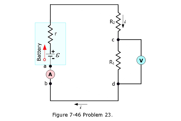
[53] In Fig. 7-46, assume that $\mathcal{E}$ = 3.0 V, r = 100 $\Omega$, $R_1$ = 250 $\Omega$, and $R_2$ = 300 $\Omega$. If the voltmeter resistance $R_V$ is 5.0 k$\Omega$, what percent error does it introduce into the measurement of the potential difference across R1? Ignore the presence of the ammeter.

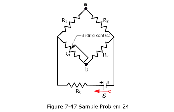
[55] In Fig. 7-47, $R_s$ is to be adjusted in value by moving the sliding contact across it until points a and b are brought to the same potential. (One tests for this condition by momentarily connecting a sensitive ammeter between a and b; if these points are at the same potential, the ammeter will not deflect.) Show that when this adjustment is made, the following relation holds: $R_x$ = $R_sR_2/R1$. An unknown resistance ($R_x$) can be measured in terms of a standard ($R_s$) using this device, which is called a Wheatstone bridge.

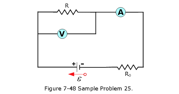
[56] In Fig. 7-48, a voltmeter of resistance $R_V$ = 300 $\Omega$ and an ammeter of resistance $R_A$ = 3.00 $\Omega$ are being used to measure a resistance R in a circuit that also contains a resistance $R_0$ = 100 $\Omega$ and an ideal battery of emf $\mathcal{E}$ = 12.0 V. Resistance R is given by R = V/i, where V is the voltmeter reading and i is the current in resistance R. However, the ammeter reading is not i but rather i’, which is i plus the current through the voltmeter. Thus, the ratio of the two meter readings is not R but only an apparent resistance R’ = V/i’. If R = 85.0 $\Omega$, what are (a) the ammeter reading, (b) the voltmeter reading, and (c) R’? (d) If $R_V$ is increased, does the difference between R’ and R increase, decrease, or remain the same?

Section 7-4 RC Circuits

[58] In an RC series circuit, emf $\mathcal{E}$ = 12.0 V, resistance R = 1.40 M$\Omega$, and capacitance C = 1.80 $\mu F$. (a) Calculate the time constant. (b) Find the maximum charge that will appear on the capacitor during charging. (c) How long does it take for the charge to build up to 16.0 $\mu C$?
[59] What multiple of the time constant t gives the time taken by an initially uncharged capacitor in an RC series circuit to be charged to 99.0% of its final charge?

	Series		Parallel
Equivalent resistance	\(R_{eq} = \sum_{j=1}^{n}R_j~\)Eq. 7.8		\(\frac{1}{R_{eq}} = \sum_{j=1}^{n}\frac{1}{R_j}~\)Eq. 7.12
Equivalent capacitor	\(\frac{1}{C_{eq}} = \sum_{j=1}^{n}\frac{1}{C_j}~\)Eq. 5.18		\(C_{eq} = \sum_{j=1}^{n}C_j~\)Eq. 5.17