Chapter 2 Electric Fields
Learning Objectives:
In this chapter you will basically learn:
\(\bullet\) Identify that a charged particle, sets up an electric field, which is a vector quantity and thus has both magnitude and direction.
\(\bullet\) Identify how an electric field \(\vec E\)can be used to explain how a charged particle can exert an electrostatic force \(\vec F\) on a second charged particle even though there is no contact between the particles.
\(\bullet\) Explain how a small positive test charge is used (in principle) to measure the electric field at any given point.
\(\bullet\) Explain electric field lines, including where they originate and terminate and what their spacing represents.
\(\bullet\) For a given point in the electric field of a charged particle, apply the relationship between the field magnitude E, the charge magnitude |q|, and the distance r between the point and the particle.
\(\bullet\) If more than one electric field is set up at a point, draw each electric field vector and then find the net electric field by adding the individual electric fields as vectors (not as scalars).
\(\bullet\) Draw an electric dipole, identifying the charges (sizes and signs), dipole axis, and direction of the electric dipole moment.
\(\bullet\) Identify the direction of the electric field at any given point along the dipole axis, including between the charges.
\(\bullet\) For an electric dipole, apply the relationship between the magnitude p of the dipole moment, the separation d between the charges, and the magnitude q of either of the charges.
\(\bullet\) For a uniform distribution of charge, find the linear charge density \(\lambda\) for charge along a line, the surface charge density \(\sigma\) for charge on a surface, and the volume charge density \(\rho\) for charge in a volume and their associated electric fields.
\(\bullet\) For a point on the central axis of a uniformly charged disk, apply the relationship between the surface charge density \(\sigma\), the disk radius R, and the distance z to that point.
\(\bullet\) For a charged particle placed in an external electric field field due to other charged objects), apply the relationship between the electric field \(\vec E\) at that point, the particle’s charge q, and the electrostatic force \(\vec F\) that acts on the particle, and identify the relative directions of the force and the field when the particle is positively charged and negatively charged.
\(\bullet\) Explain Millikan’s procedure of measuring the elementary charge and also explain the general mechanism of ink-jet printing.
\(\bullet\) Calculate the torque on an electric dipole in an external electric field and relate the potential energy of the dipole to the work done by a torque as the dipole rotates in the electric field.
2.1 The Electric Field:
A temperature field and pressure field are scalar fields because temperature and pressure, having only magnitudes and no directions are associated with these fields. On the other hand electric field is a vector field with direction similar to gravitational field. Electric field can be directed inward or outward but gravitational field \(\vec g\) is directed inward towards the Earth.
\[\begin{equation} \vec{g} = \vec{F}/m \tag{2.1} \end{equation}\]
We can measure the gravitational force \(\vec F\) at point P on a point mass, m due to the Earth’s gravitational field \(\vec g\) as shown in Fig. 2-1a. Analogously, we can measure the electrostatic force at point P that acts on the test charge \(q_{0}\) due to a charged object as shown in Fig. 2-1b and 2-1b. Basic assumption is that the charge must be small so that it does not disturb the object’s charge distribution. The electric field at that point is then is given by:
\[\begin{equation} \vec{E} = \vec{F}/q_{0} \tag{2.2} \end{equation}\]
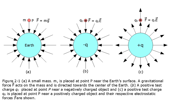
The SI unit for the gravitational field can be seen from Eq. 2-1 is the newton per kg (N/kg).
Since the test charge \(q_0\) is positive, the two vectors in Eq. 2-2 are in the same direction, so the direction of \(\vec{E}\) is the direction we measure for \(\vec{F}\).The magnitude of \(\vec{E}\) at point P is \(F/q_{0}\). As shown in Fig. 2-1b and 2-1c, we always represent an electric field with an arrow with its tail anchored on the point where the measurement is made. The SI unit for the electric field can be seen from Eq. 2-2 is the newton per coulomb (N/C).
A positive test charge at any point near the negatively chaged sphere as shown in Fig. 2-1b, we find that an electrostatic force pulls on it toward the center of the sphere. Thus at every point around the sphere, an electric field vector points radially inward toward the sphere. Similarly, a positive test charge at any point near the positively chaged sphere as shown in Fig. 2-1c, we find that an electrostatic force pushes on it outward the center of the sphere. Thus at every point around the sphere, an electric field vector points radially outward away from the sphere.
2.2 Electric Field Lines:
In Fig. 2-2 shows a side view of an infinitely large, nonconducting sheet (or plane) with a uniform distribution of positive charge on one side. If we place a positive test charge at any point near the sheet (on either side), we find that the electrostatic force on the particle is outward and perpendicular to the sheet.
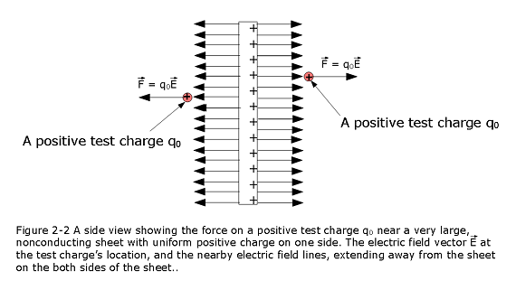
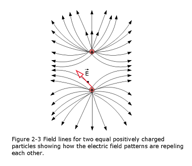
Figure 2-3 shows the field lines for two particles with equal positive charges. Now the field lines are curved, but the rules still hold: (1) the electric field vector at any given point must be tangent to the field line at that point and in the same direction, as shown for one vector, and (2) a closer spacing means a larger field magnitude.
2.3 The Electric Field Due to a Point Charge:
To find the electric field due to a charged particle (often called a point charge),we place a positive test charge at any point near the particle, at distance r. From Coulomb’s law (Eq.2-1),the force on the test charge due to the particle with charge q is
\[\begin{equation} \vec{F}=\frac{1}{4\pi\varepsilon_{0}}\frac{qq_{0}}{r^2}\hat{r} \tag{2.3} \end{equation}\]
As previously, the direction of \(\vec{F}\) is directly away from the particle if q is positive (because \(q_0\) is positive) and directly toward it if q is negative. Using Eq. 3-1, we can express the electric field set up by the particle (at the location of the test charge) is given by
\[\begin{equation} \vec{E} = \vec{F}/q_{0} = \frac{1}{4\pi\varepsilon_{0}}\frac{q}{r^2}\hat{r} \tag{2.4} \end{equation}\]
The magnitude at any given distance r is given by: \[\begin{equation} E = \frac{1}{4\pi\varepsilon_{0}}\frac{|q|}{r^2} (charged\space particle) \tag{2.5} \end{equation}\]
In general, if several electric fields are set up at a given point by several charged particles, we can find the net field by placing a positive test particle at the point using superposition principle, so we just add the fields as vectors:
\[\begin{equation} \vec{E} = \vec{F}_{01}/q_0 + \vec{F}_{02}/q_0 + ........+ \vec{F}_{0n}/q_0 = \vec{E}_{1} + \vec{E}_{2} + ........+ \vec{E}_{n} \tag{2.6} \end{equation}\]
2.4 The Electric Field Due to an Electric Dipole:
An electric dipole is shown in Figure 2-4 shows the pattern of electric field lines for two charged particles that have the same charge magnitude q but opposite signs.
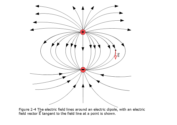
Python-code generated electric field lines of a dipole using python libraries of Thomas J. Duck (https://github.com/tomduck/electrostatics/).
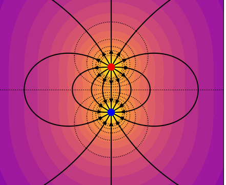
Figure 2-5 shows the electric fields set up at P by each particle. The nearer particle
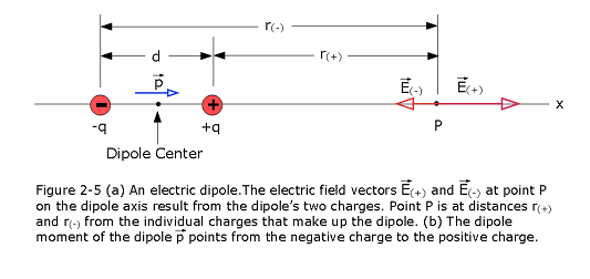
with charge +q sets up field \(E_{(+)}\) in the positive direction of the x axis (directly away from the particle). The farther particle with charge -q sets up a smaller field \(E_{(-)}\) in the negative direction (directly toward the particle). We want the net field at P. However, because the field vectors are along the same axis, let’s simply indicate the vector directions with plus and minus signs, as we commonly do with forces along a single axis. Then we can write the magnitude of the net field at P as
\[\begin{equation} E = E_{(+)} + E_{(-)} = \frac{1}{4\pi\varepsilon_{0}}\frac{q}{r_{(+)}^2} - \frac{1}{4\pi\varepsilon_{0}}\frac{q}{r_{(-)}^2} = \frac{1}{4\pi\varepsilon_{0}}\frac{q}{(x-d/2)^2} - \frac{1}{4\pi\varepsilon_{0}}\frac{q}{(x+d/2)^2} \tag{2.7} \end{equation}\]
Taking x out of the parentheses, we can rewrite this equation as
\[\begin{equation} E = \frac{q}{4\pi\varepsilon_{0}{x^2}}{\left(\frac{1}{{(1-d/xz)^2}} - \frac{1}{{(1+d/2x)^2}}\right)} \tag{2.8} \end{equation}\]
After forming a common denominator and multiplying its terms, we come up with the following expression
\[\begin{equation} E = \frac{q}{4\pi\varepsilon_{0}{x^2}}\frac{2d/x}{\left(1-(d/2x)^2\right)^2} \tag{2.9} \end{equation}\]
At x >> d such that \(\frac{d}{2x} << 1\) in Eq. 2-8.Thus, in our approximation, we can neglect the \(\frac{d}{2x}\) term in the denominator, which leaves us with
\[\begin{equation} E = \frac{qd}{2\pi\varepsilon_{0}{x^3}} \tag{2.10} \end{equation}\]
The product qd, which involves the two intrinsic properties q and d of the dipole, is the magnitude p of a vector quantity known as the electric dipole moment \(\vec p\) of the dipole.(The unit of \(\vec p\) is the coulomb-meter.) Thus, we can rewrite Eq. 2-9 as follows:
\[\begin{equation} E = \frac{p}{2\pi\varepsilon_{0}{x^3}}\space (electric \space dipole) \tag{2.11} \end{equation}\]
2.5 The Electric Field Due to a Line of Charge:
Figure 2-6 shows a thin ring of radius R with a uniform distribution of positive charge along its circumference. It is made of plastic, which means that the charge is fixed in place.The ring is surrounded by a pattern of electric field lines, but here we restrict our interest to an arbitrary point P on the central axis (the axis through the ring’s center and perpendicular to the plane of the ring), at distance z from the center point. The charge of an extended object is often conveyed in terms of a charge density rather than the total charge. For a line of charge, we use the linear charge density \(\lambda\) (the charge per unit length), with the SI unit of coulomb per meter. Similarly, Table 2-1 shows the other charge densities, surface charge density, \(\sigma\) (the charge per unit area), volume charge density \(\rho\) (the charge per unit volume) that we shall be using for charged surfaces and volumes in the sections ahead of this section.
Table 2-1 Particle, Symbol and Charge.
| Name | Symbol | SI Unit |
|---|---|---|
| Charge | q | \(C\) |
| Linear Charge Density | \(\lambda\) | \(C/m\) |
| Surface Charge Density | \(\sigma\) | \(C/m^2\) |
| Volume Charge Density | \(\rho\) | \(C/m^3\) |
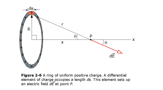
We arbitrarily pick the charge element shown in Fig. 2-6. Let ds be the arc length of that (or any other) dq element.Then in terms of the linear density \(\lambda\) (the charge per unit length), we have
\[\begin{equation} dq = \lambda ds \tag{2.12} \end{equation}\]
This charge element sets up the differential electric \(d\vec{E}\) field at P, at distance r from the element, as shown in Fig. 2-6. The field magnitude dE due to the charge element dq is
\[\begin{equation} dE = \frac{dq}{4\pi\varepsilon_{0}{r^2}}= \frac{\lambda ds}{4\pi\varepsilon_{0}{(x^2 + R^2)}} \tag{2.13} \end{equation}\]
The differential field \(\vec{E}\) has \(sin\theta\) components that cancel each other but the \(cos\theta\) contributes as can be seen in Fig. 22-12.
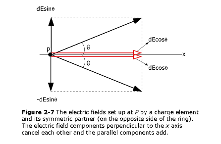
Using right triangle rule we can replace \(cos\theta\) as follows:
\[\begin{equation} cos\theta = \frac{x}{r} = \frac{x}{\sqrt{(x^2 + R^2)}} \tag{2.14} \end{equation}\]
Multiplying Eq. 2-12 by Eq. 2-13 gives us the parallel field component from each charge element:
\[\begin{equation} dE\cos\theta = \frac{\lambda ds}{4\pi\varepsilon_{0}{(x^2 + R^2)}}\frac{x}{\sqrt{(x^2 + R^2)}} \tag{2.15} \end{equation}\]
By integrating along the ring,from a starting point (s = 0) through the full circumference (\(s = 2\pi R\)) we get the total electric field of a non-conducting charged ring at a point P on the central axis (the axis through the ring’s center and perpendicular to the plane of the ring), at distance x from the center point.
\[\begin{equation} E=\frac{\lambda x}{4\pi\varepsilon_{0}(x^2 + R^2)^{3/2}}\int_0^{2\pi R}ds =\frac{2 \pi R\lambda x}{4\pi\varepsilon_{0}(x^2 + R^2)^{3/2}} \tag{2.16} \end{equation}\]
\[\begin{equation} E= \frac{qx}{4\pi\varepsilon_{0}(x^2 + R^2)^{3/2}} (charged \space ring) \tag{2.17} \end{equation}\]
If the charge on the ring is negative, instead of positive as we have assumed, the magnitude of the field at P is still given by Eq. 2-16. However, the electric field vector then points toward the ring instead of away from it.
Let us check Eq. 2-16 for a point on the central axis that is so far away that x >> R. \[\begin{equation} E= \frac{1}{4\pi\varepsilon_{0}}\frac{q}{x^2} (charged \space ring \space at \space large \space distance) \tag{2.18} \end{equation}\]
The result in Eq. 2-17 is for a point charge if we replace x with r in Eq. 2-17, as given by Eq. 22-3.
2.6 The Electric Field Due to a Charged Disk:
Now we calculate the electric field of a circular plastic disk, with a radius R and a uniform surface charge density \(\sigma\) (charge per unit area, Table 22-1) on its top surface. The electric field at an arbitrary point P on the central axis, at distance z from the center of the disk, as indicated in Fig. 2-8.
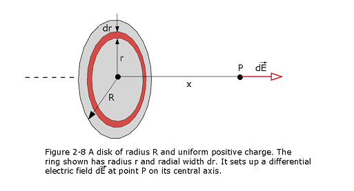
A disk is basically consists of many rings for which we already have result as given in Eq. 2-16. We can find the electric field at a point P on the central axis, at a distance z from the center of the disk by integrating the Eq. 2-16 from its center r = 0 to r = R of the disk.
\[\begin{equation} dE= \frac{dq\space x}{4\pi\varepsilon_{0}(x^2 + r^2)^{3/2}} \tag{2.19} \end{equation}\]
We can replace dq, in terms of the surface charge density \(\sigma\), as follows
\[\begin{equation} dq = \sigma dA = \sigma(2\pi r \space dr) \tag{2.20} \end{equation}\]
\[\begin{equation} E = \int dE = \frac{\sigma x}{4\varepsilon_{0}}\int_0^R(x^2 + r^2)^{-3/2}(2r)dr \tag{2.21} \end{equation}\]
Using standard integral, \[\begin{equation} \int X^{m}dX = \frac{X^{m+1}}{m+1} \tag{2.22} \end{equation}\]
and substituting \(X = (x^2 + r^2)\) and \(m=-\frac{3}{2}\) and \(dX = (2r)dr\), we get
\[\begin{equation} E = \frac{\sigma x}{4\varepsilon_{0}}\left[\frac{(x^2 + r^2)^{-1/2}}{-1/2}\right]_{0}^{R} \tag{2.23} \end{equation}\]
\[\begin{equation} E = \frac{\sigma}{2\varepsilon_{0}}\left[1-\frac{x}{\sqrt{x^2 + R^2}}\right](charged\space disk) \tag{2.24} \end{equation}\]
If we let \({R \to \infty}\) while keeping x finite, the second term in the parentheses in Eq. 22-23 approaches zero, and this equation reduces to
\[\begin{equation} E = \frac{\sigma}{2\varepsilon_{0}}(infinite\space sheet) \tag{2.25} \end{equation}\]
This is the electric field produced by an infinite sheet of uniform charge located on one side of a nonconductor such as plastic.
Example Problem 2.01 Net electric field due to three charged particles Figure 2-9a shows three particles with charges \(q_1\) = +2Q, \(q_2\) = -2Q, and \(q_3\) = -4Q, each a distance d from the origin. What net electric field is produced at the origin?
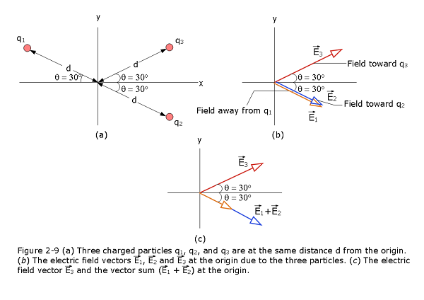
Magnitudes and directions: To find the magnitude of \(E_1\) which is due to \(q_1\), we use Eq. 3-4, substituting d for r and 2Q for q and obtaining
\(E_1 = \frac{1}{4\pi\varepsilon_{0}}\frac{2Q}{d^2}\) To find the magnitude of \(E_2\) which is due to \(q_2\), we use Eq. 3-4, substituting d for r and 2Q for q and obtaining
\(E_2 = \frac{1}{4\pi\varepsilon_{0}}\frac{2Q}{d^2}\) To find the magnitude of \(E_3\) which is due to \(q_3\), we use Eq. 3-4, substituting d for r and 4Q for q and obtaining
\(E_3 = \frac{1}{4\pi\varepsilon_{0}}\frac{4Q}{d^2}\)
Adding the fields:
\(E_1 + E_2\) = \(\frac{1}{4\pi\varepsilon_{0}}\frac{2Q}{d^2} + \frac{1}{4\pi\varepsilon_{0}}\frac{2Q}{d^2} = \frac{1}{4\pi\varepsilon_{0}}\frac{4Q}{d^2}\)
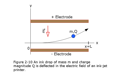
Example Problem 2.02 Motion of a charged particle in an electric field
Figure 2-10 shows the deflecting plates of an ink-jet printer, with superimposed coordinate axes. An ink drop with a mass m of \(1.3 \times 10^{-10}\) kg and a negative charge of magnitude \(Q = 1.5 \times 10^{-13}\) C enters the region between the plates, initially moving along the x axis with speed \(v_x = 18\) m/s. The length L of each plate is 1.6 cm. The plates are charged and thus produce an electric field at all points between them. Assume that field \(\vec E\) is downward directed, is uniform, and has a magnitude of \(1.4 \times 10^6\) N/C. What is the vertical deflection of the drop at the far edge of the plates? (The gravitational force on the drop is small relative to the electrostatic force acting on the drop and can be neglected.)
Solution:
Using Newton’s second law (F = ma) for components along along the y-axis we get
\[a_y = \frac{F}{m}=\frac{QE}{m}\] Let t represent the time required for the drop to pass through the region between the plates. During t the vertical and horizontal displacements of the drop are
\(y = \frac{1}{2}a_y t^2\) and \(L = v_xt\), respectively.
Eliminating t between the above two equations and substituting \(a_y\),we find
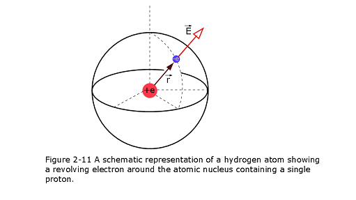
\[y = \frac{QEL^2}{2mv_x^2}= \frac{(1.5 \times 10^{-13}C)(1.4 \times 10^6N/C)(1.6\times 10^{-2} m)^2}{2(1.3 \times 10^{-10}kg)(18m/s)^2}=6.4\times 10^{-4}\space m (Answer)\] Example Problem 2.03 In an ionized hydrogen atom, the distance between the nucleus and the electron is \(r=5.292\times10^{-11}~{m}\). What is the electric field due to the nucleus at the location of the electron?
Solution:
\[\vec E=\frac{1}{4\pi\varepsilon_{0}}\frac{e}{r^2}\hat r=\left({8.99 \times 10^9}{\frac{N.m^2}{C^2}}\right)\frac{1.6\times 10^{-19}\space C}{(5.292\times 10^{-11}\space m)^2}\hat r =5.14\times 10^{11}\space N/C\space\hat r (Answer)\] The direction of \(\vec E\) is radially outward from the nucleus in all directions.
Solved Problems Electric Fields
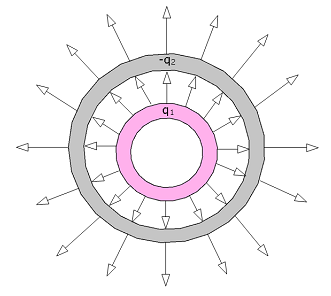
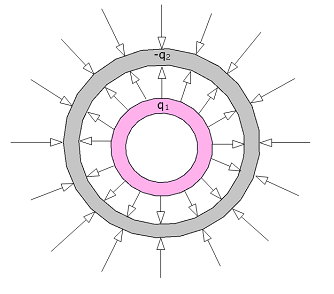
- [1] Sketch qualitatively the electric field lines both between and outside two concentric conducting spherical shells when a uniform positive charge \(q_1\) is on the inner shell and a uniform negative charge \(-q_2\) is on the outer. Consider the cases \(q_1 \gt q_2\), \(q_1 = q_2\), and \(q_1 \lt q_2\).
Solution:
Electric field pattern due to charge in the inner shell is greater than the charge on the outer shell (\(q_1 = q_2\))
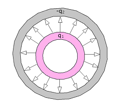
Electric field pattern due to charge in the inner shell is greater than the charge on the outer shell (\(q_1 \gt q_2\))
Electric field pattern due to charge in the inner shell is greater than the charge on the outer shell (\(q_1 \lt q_2\))
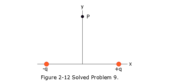
- [9] Figure 2-12 shows two charged particles on an x axis: \(-q = -3.20 \times 10^{-19}\) C at x = -3.00 m and \(q = 3.20 \times 10^{-19}\) C at x = +3.00 m. What are the (a) magnitude and (b) direction (relative to the positive direction of the x axis) of the net electric field produced at point P at y = 4.00 m?
Solution:
- Figure 2-12 can be redrawn showing the electric fields and other given dimensions as shown below:
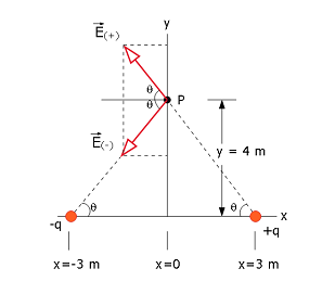
It can be seen that the vertical components (y-components) of the electric fields cancel each other due to symmetry. The horizontal components (x-components) add together along the negative x-axis will contribute to the net electric field:
\[E_{net}=E_{(+)}+E_{(-)}=2E\cos\theta=\frac{2}{4\pi\varepsilon_{0}}\frac{|q|}{r^2}\cos\theta=\frac{2}{4\pi\varepsilon_{0}}\frac{|q|}{(x^2+y^2)}\frac{x}{\sqrt{(x^2+y^2)}}=\frac{2}{4\pi\epsilon_{0}}\frac{|q|x}{(x^2+y^2)^{3/2}}\] \[E_{net}=\frac{1}{4\pi\varepsilon_{0}}\frac{2|q|x}{(x^2+y^2)^{3/2}}\] \[E_{net}==\left({8.99 \times 10^9}{\frac{N.m^2}{C^2}}\right)\frac{2|\pm 3.20 \times 10^{-19}\space C||\pm3\space m|}{(3^2\space m^2+4^2\space m^2)^{3/2}}=1.38\times 10^{-10}\space N/C\space (Answer)\] (b) Direction is \(180^\circ\) from the +x-axis or along the negative x-axis. (Answer)
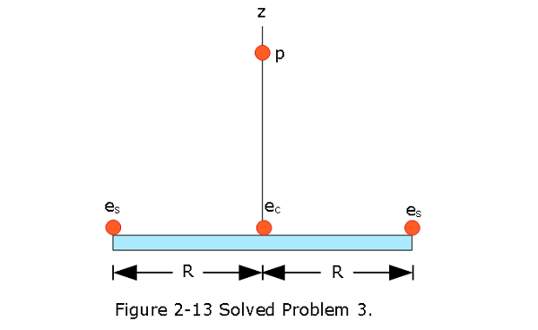
- [13] Figure 2-13 shows a proton (p) on the central axis through a disk with a uniform charge density due to excess electrons.The disk is seen from an edge-on view. Three of those electrons are shown: electron \(e_c\) at the disk center and electrons \(e_s\) at opposite sides of the disk, at radius R from the center. The proton is initially at distance z = R = 2.00 cm from the disk. At that location, what are the magnitudes of (a) the electric field \(\vec E_c\) due to electron \(e_c\) and (b) the net electric field \(\vec E_{s,net}\) due to electrons \(e_s\)? The proton is then moved to z = R/10.0. What then are the magnitudes of (c) \(\vec E_c\) and (d) \(\vec E_{s,net}\) at the proton’s location? (e) From (a) and (c) we see that as the proton gets nearer to the disk, the magnitude of \(\vec E_c\) increases, as expected. Why does the magnitude of \(\vec E_{s,net}\) from the two side electrons decrease, as we see from (b) and (d)?
Solution:
- The magnitude of the electric field \(\vec E_c\) at point z = r = \(2.00\times 10^{-2}\space m\) due to electron an \(e_c\) is:
\[E_c=\frac{1}{4\pi\varepsilon_{0}}\frac{e}{r^2}=\left({8.99 \times 10^9}{\frac{N.m^2}{C^2}}\right)\frac{1.6\times 10^{-19}\space C}{(2.00\times 10^{-2}\space m)^2}=3.596\times 10^{-6}\space N/C\space (Answer)\] (b) The net electric field \(\vec E_{s,net}\) due to electrons \(e_s\) can be found using the following figure.
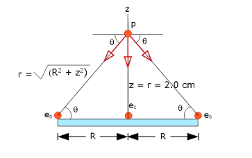
It can be seen from the figure that the horizontal components of the forces cancel each other but the vertical components directed downward will contribute as the net force. Thus,
\[E_{s,net}=2E_s\sin\theta=\frac{2}{4\pi\varepsilon_{0}}\frac{e}{r^2}\sin\theta=\frac{1}{4\pi\varepsilon_{0}}\frac {2ez}{(R^2+z^2)^{3/2}}\] \[E_{s,net}=\frac{1}{4\pi\varepsilon_{0}}\frac {2ez}{(R^2+z^2)^{3/2}}\] \[E_{s,net}=\left({8.99 \times 10^9}{\frac{N.m^2}{C^2}}\right)\frac{2\times 1.6\times 10^{-19}\space C\times 2.00\times 10^{-2}\space m}{((2.00\times 10^{-2}\space m)^2+(2.00\times 10^{-2}\space m)^2)^{3/2}}\]
\[E_{s,net}=2.543\times 10^{-6}\space N/C\space (Answer)\] (c) The proton is then moved to z = R/10.0. What then are the magnitudes of \(\vec E_c\)
\[E_c=\frac{1}{4\pi\varepsilon_{0}}\frac{e}{r^2}=\left({8.99 \times 10^9}{\frac{N.m^2}{C^2}}\right)\frac{1.6\times 10^{-19}\space C}{(2.00\times 10^{-3}\space m)^2}=3.596\times 10^{-4}\space N/C\space (Answer)\]
- The proton is then moved to z = R/10.0. What then is the magnitude of \(\vec E_{s,net}\) at the proton’s location?
\[E_{s,net}=\frac{1}{4\pi\varepsilon_{0}}\frac {2ez}{(R^2+z^2)^{3/2}}\]
\[E_{s,net}=\left({8.99 \times 10^9}{\frac{N.m^2}{C^2}}\right)\frac{2\times 1.6\times 10^{-19}\space C\times 2.00\times 10^{-2}\space m}{((2.00\times 10^{-2}\space m)^2+(2.00\times 10^{-3}\space m)^2)^{3/2}}\]
\[E_{s,net}=7.085\times 10^{-6}\space N/C\space (Answer)\]
- In part (c) \(E_c\) is inversely proportional to \(z_2\), but for part (d) it is propostional to \(\frac {z}{(R^2+z^2)^{3/2}}\), and as a result \(\vec E_c\) increases, and \(\vec E_{s,net}\) decreases.
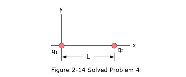
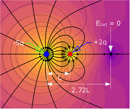
- [14] In Fig. 2-14, particle 1 of charge \(q_1 = -5.00q\) and particle 2 of charge \(q_2 = +2.00q\) are fixed to an x axis. (a) As a multiple of distance L, at what coordinate on the axis is the net electric field of the particles zero? (b) Sketch the net electric field lines between and around the particles.
Solution:
- There is a point on the right side of the charged particles where the net electric field is zero as can be seen in the figure below. Thus, we can write
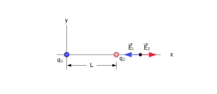
\[\vec E_{net} = \vec E_2-\vec E_1=0\] Therefore, in terms of magnitudes, we can write \[\frac{1}{4\pi\varepsilon_{0}}\frac{|q_1|}{x^2}=\frac{1}{4\pi\varepsilon_{0}}\frac{|q_2|}{(x-L)^2}\] \[\frac{1}{4\pi\varepsilon_{0}}\frac{|-5q|}{x^2}=\frac{1}{4\pi\varepsilon_{0}}\frac{|+2q|}{(x-L)^2}\] \[\frac{x-L}{x}=\sqrt{\frac{2}{5}}\] \[x=\frac{L}{1-\sqrt{\frac{2}{5}}}=2.721L\space (Answer)\] (b) Python-code generated electric field lines between and around the particles using python libraries of Thomas J. Duck (https://github.com/tomduck/electrostatics/).
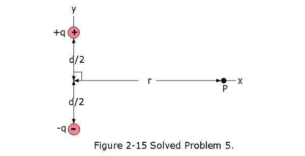
- [19] Figure 2-15 shows an electric dipole. What are the (a) magnitude and (b) direction (relative to the positive direction of the x axis) of the dipole’s electric field at point P, located at distance \(r \gg d\)?
Solution: (a) To find the electric dipole at P, it is useful to draw the electric field vectors as shown in the figure below:
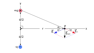
\[\vec E_{net}=\vec E_{+}+\vec E_{-}\] Resolving along the x direction we get, \[E_{net,x}= E\cos\theta-E\cos\theta=0\],
since the magnitudes of \(E_{+}=E_{-}=E\).
Similarly, resolving along the y direction we get, \[E_{net,y}= -E\sin\theta-E\sin\theta=-2E\sin\theta=-\frac{2}{4\pi\varepsilon_{0}}\frac{q}{(\frac{d}{2})^2+r^2}\frac{d/2}{\sqrt{(\frac{d}{2})^2+r^2}}\] The magnitude of the net electric field becomes,
\[\left|E_{net,y}\right|=\left|-\frac{1}{4\pi\varepsilon_{0}}\frac{qd}{\left[(\frac{d}{2})^2+r^2\right]^{3/2}}\right|=\frac{1}{4\pi\varepsilon_{0}}\frac{qd}{\left[(\frac{d}{2})^2+r^2\right]^{3/2}}\] The approximate value of the \(\left|E_{net,y}\right|\) when \(r \gg d\) becomes
\[\left|E_{net,y}\right|=\frac{1}{4\pi\varepsilon_{0}}\frac{qd}{\left[(\frac{d}{2})^2+r^2\right]^{3/2}}=\frac{1}{4\pi\varepsilon_{0}}\frac{qd}{r^3\left[(\frac{d}{2r})^2+1\right]^{3/2}}\approx \frac{1}{4\pi\varepsilon_{0}}\frac{qd}{r^3}\space (Answer)\] (b) The \(|E_{net,y}|\) is directed along the negative y-axis or along \(-\hat j\) direction, and \(-90^\circ\) from the +x axis.
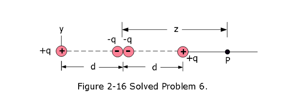
- [21] Electric quadrupole. Figure 2-16 shows a generic electric quadrupole. It consists of two dipoles with dipole moments that are equal in magnitude but opposite in direction. Show that the value of E on the axis of the quadrupole for a point P a distance z from its center (assume \(z \gg d\)) is given by \[E=\frac{3Q}{4\pi\varepsilon_0z^4}\] in which Q (\(=2qd^2\)) is known as the quadrupole moment of the charge distribution.
Solution:
Electric fields at point P due to four charges can be added to find the result as follows:
\[E_{net}=\frac{1}{4\pi\varepsilon_{0}}\frac{q}{(z-d)^2}-\frac{1}{4\pi\varepsilon_{0}}\frac{2q}{z^2}+\frac{1}{4\pi\varepsilon_{0}}\frac{q}{(z+d)^2}\] \[E_{net}=\frac{q}{4\pi\varepsilon_{0}}\frac{(1-d/z)^{-2}}{z^2}-\frac{1}{4\pi\varepsilon_{0}}\frac{2q}{z^2}+\frac{q}{4\pi\varepsilon_{0}}\frac{(1+d/z)^{-2}}{z^2}\] Using Binomial expansion, \[(1+x)^n=1 + nx +\frac{n(n-1)x^2}{2!}+\frac{n(n-1)(n-2)x^3}{3!}+.....\] we can expand \[(1-d/z)^{-2}\approx 1+\frac{2d}{z}+\frac{6d^2}{2z^2}+....\]
and \[(1+d/z)^{-2}\approx 1-\frac{2d}{z}+\frac{6d^2}{2z^2}+....\]
Therefore, we can write \[E_{net}\approx \frac{q}{4\pi\varepsilon_{0}z^2}\left(1+\frac{2d}{z}+\frac{6d^2}{2z^2}\right)-\frac{1}{4\pi\varepsilon_{0}}\frac{2q}{z^2}+\frac{q}{4\pi\varepsilon_{0}z^2}\left(1-\frac{2d}{z}+\frac{6d^2}{2z^2}\right)\] Cancelling terms we get, \[E_{net}\approx \frac{1}{4\pi\varepsilon_{0}}\frac{6qd^2}{z^4}=\frac{1}{4\pi\varepsilon_{0}}\frac{3Q}{z^4}\space (Answer)\] where we have made use \(Q = 2qd^2\) as the quadrupole moment.
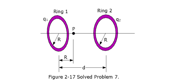
- [23] Figure 2-17 shows two parallel nonconducting rings with their central axes along a common line. Ring 1 has uniform charge \(q_1\) and radius R; ring 2 has uniform charge \(q_2\) and the same radius R. The rings are separated by distance d = 3.00R.The net electric field at point P on the common line, at distance R from ring 1, is zero. What is the ratio \(q_1/q_2\)?
Solution:
Using Eqn 3-16, and applyinng the given condition that the net electric field at point P on the common line, at distance R from ring 1, is zero, we can write,
\[E_{left-ring}= \frac{qx}{4\pi\varepsilon_{0}(x^2 + R^2)^{3/2}}=\frac{q_1R}{4\pi\varepsilon_{0}(R^2 + R^2)^{3/2}}\] \[E_{right-ring}= \frac{qx}{4\pi\varepsilon_{0}(x^2 + R^2)^{3/2}}=\frac{q_2(2R)}{4\pi\varepsilon_{0}\left[(2R)^2 + R^2\right]^{3/2}}\] \[E_{left-ring}=E_{right-ring}\] \[\frac{q_1R}{4\pi\varepsilon_{0}(R^2 + R^2)^{3/2}}=\frac{q_2(2R)}{4\pi\varepsilon_{0}\left[(2R)^2 + R^2\right]^{3/2}}\] \[\frac{q_1}{q_2}=\frac{2(2R^2)^{3/2}}{(5R^2)^{3/2}}=2\left(\frac{2}{5}\right)^{3/2}=0.506\space (Answer)\]
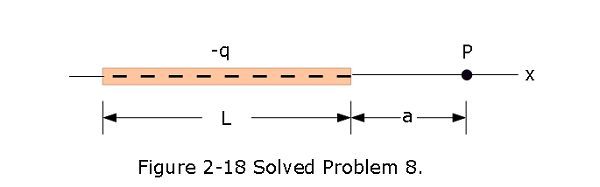
- [31] In Fig. 2-18, a nonconducting rod of length L = 8.15 cm has a charge -q = -4.23 fC uniformly distributed along its length. (a) What is the linear charge density of the rod? What are the (b) magnitude and (c) direction (relative to the positive direction of the x axis) of the electric field produced at point P, at distance a = 12.0 cm from the rod? What is the electric field magnitude produced at distance a = 50 m by (d) the rod and (e) a particle of charge -q = -4.23 fC that we use to replace the rod? (At that distance, the rod “looks” like a particle.)
Solution:
- Linear charge density \(\lambda = \frac{q}{L}\space (C/m)\) \[\lambda = \frac{q}{L}=\frac{-4.23 \times 10^{-15}\space C}{8.15\times 10^{-2}\space m}=-5.2\times 10^{-14}\space C/m\space (Answer)\]
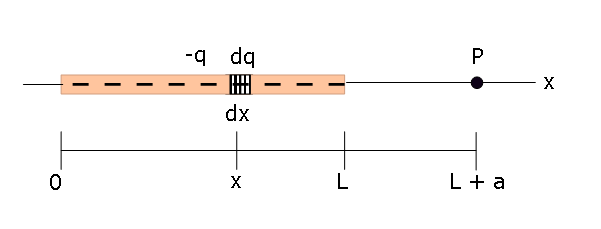
- To calculate the magnitude of the electric field produced at point P, we consider a differential amount of charge \(dq\) with its corresponding differential element dx as shown in the figure below:
The differential electric field component at point P becomes,
\[dE_x = \frac{1}{4\pi\varepsilon_{0}}\frac{dq}{r^2}=\frac{1}{4\pi\varepsilon_{0}}\frac{\lambda dx}{(L+a-x)^2}\] Therefore, the total electric field can be calculated by integrating from 0 to L over which the charge is extended.
\[E_x = \left.\frac{\lambda}{4\pi\epsilon_{0}}\int_0^L\frac{ dx}{(L+a-x)^2}=\frac{\lambda}{4\pi\epsilon_{0}}\frac{1}{(L+a-x)}\right\vert _0^L=\frac{\lambda}{4\pi\epsilon_{0}}\left[\frac{1}{a}-\frac{1}{L+a}\right]\] \[E_x =\frac{\lambda }{4\pi\varepsilon_{0}}\left[\frac{L}{a(L+a)}\right]=-\frac{1 }{4\pi\varepsilon_{0}}\left[\frac{q}{a(L+a)}\right]\] where we made use \(\lambda = \frac{q}{L}\) to get the final expression. Thus, the magnitude of the electric field
\[|E_x| = \left\vert -\frac{1 }{4\pi\varepsilon_{0}}\left(\frac{q}{a(L+a)}\right)\right\vert =\left\vert\left({8.99 \times 10^9}{\frac{N.m^2}{C^2}}\right)\left(\frac{-4.23 \times 10^{-15}\space C}{(0.120\space m)(0.0815\space m+0.120\space m)}\right)\right\vert\] \[|E_x|=\left\vert\left({8.99 \times 10^9}{\frac{N.m^2}{C^2}}\right)\left(\frac{-4.23 \times 10^{-15}\space C}{(0.120\space m)(0.0815\space m+0.120\space m)}\right)\right\vert =1.577\times 10^{-3}\space N/C\space (Answer)\] (c) The direction of the field relative to the positive direction of the x axis is \(-180^\circ\) or along the -x axis.
\[|E_x|=\Big|\left({8.99 \times 10^9}{\frac{N.m^2}{C^2}}\right)\left(\frac{-4.23 \times 10^{-15}\space C}{(50\space m)(0.0815\space m+50\space m)}\right)\Big |\approx 1.52\times 10^{-8}\space N/C\space (Answer)\]
Replacing the rod with a particle of charge -q = -4.23 fC the electric field is same as in part (d) that is \(|E_x| \approx 1.52\times 10^{-8}\space N/C\space (Answer)\)
If \(a\gg L\), we can neglect L and as a result the electric field becomes
\[E_x =\frac{\lambda }{4\pi\varepsilon_{0}}\left[\frac{L}{a(L+a)}\right]\approx -\frac{1 }{4\pi\varepsilon_{0}}\left[\frac{q}{a^2}\right]\] and the line can be replaced by a point charge and the result becomes same as (d).
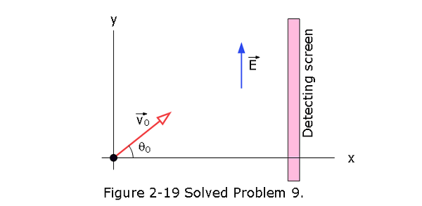
- [54] In Fig. 2-19, an electron is shot at an initial speed of \(v_0 = 2.00 \times 10^6\) m/s, at angle \(\theta_0 = 40^\circ\) from an x axis. It moves through a uniform electric field \(\vec E = (5.00\space N/C)\hat j\)$. A screen for detecting electrons is positioned parallel to the y axis, at distance x = 3.00 m. In unit-vector notation, what is the velocity of the electron when it hits the screen?
Solution:
It is basically a projectile motion, we need the find the x and y components of velocities to find the resultant velocity.
The x-component of the velocity can be calculated using \[v_x = v_0\cos\theta_0=(2.00 \times 10^6\space m/s)\cos40^\circ=1.53\times 10^6\space m/s\] The y-component of the velocity can be calculated using \[v_y = v_0\sin\theta_0-at\] However, we need to calculate the time it takes to hit the screen which is x = 3 m away
\[t = \frac{x}{v_0\cos\theta_0}=\frac{3\space m}{(2.00 \times 10^6\space m/s)\cos40^\circ}=1.958\times 10^{-6}\space s\] We also need to calculate acceleration a to calculate \(v_y\) \[a = \frac{eE}{m}=\frac{1.6\times 10^{-19}\space C (5.00\space N/C)}{9.1\times 10^{-31}\space kg}=8.79\times 10^{11}\space m/s^2\] \[v_y = v_0\sin\theta_0-at=(2.00 \times 10^6\space m/s)\sin40^\circ-(8.79\times 10^{11}\space m/s^2)(1.958\times 10^{-6}\space s)=\] \[v_y = (2.00 \times 10^6\space m/s)\sin40^\circ-(8.79\times 10^{11}\space m/s^2)(1.958\times 10^{-6}\space s)=-4.35\times 10^5\space m/s\] In unit-vector notation, the velocity of the electron when it hits the screen becomes
\[\vec v = 1.53\times 10^6\space m/s\space \hat i-4.35\times 10^5\space m/s\space \hat j\space (Answer)\] 10. [78] Two particles, each of positive charge q, are fixed in place on a y axis, one at y = d and the other at y = -d. (a) Write an expression that gives the magnitude E of the net electric field at points on the x axis given by \(x = \alpha d\). (b) Graph E versus \(\alpha\) for the range \(0 \lt \alpha \lt 4\). From the graph, determine the values of \(\alpha\) that give (c) the maximum value of E and (d) half the maximum value of E.
Solution:
To solve this prolem it is helpful to visualize the problem using the following figure.
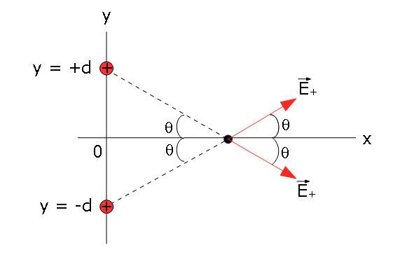
From the above figure we can immediately see that the y-components of the fields cancel each other. On the x-components add together.
\[\vec E_{net}=\vec E_{(+)} + \vec E_{(+)}\] \[E_{net,y}= E\sin\theta - E\sin\theta=0\] \[E_{net,x}= E\cos\theta + E\cos\theta = 2E\cos\theta\] \[E_{net,x} = 2E\cos\theta=\frac{2}{4\pi\varepsilon_{0}}\frac{q}{r^2}\frac{\alpha d}{r}=2\left({8.99 \times 10^9}{\frac{N.m^2}{C^2}}\right)\frac{q}{r^2}\] \[E_{net,x}=\frac{q}{2\pi\varepsilon_{0}}\frac{1}{(d^2+\alpha^2d^2)}\frac{\alpha d}{\sqrt{(d^2+\alpha^2d^2)}}\] \[E_{net,x}=\frac{q}{2\pi\varepsilon_{0}d^2}\left[\frac{\alpha}{(1+\alpha^2)^{3/2}}\right]\] \[E_{net,x}\propto \frac{\alpha}{(1+\alpha^2)^{3/2}}\] since \(\frac{q}{2\pi\varepsilon_{0}d^2}\) is a scalar.
- Graph E versus \(\alpha\) for the range \(0 \lt \alpha \lt 4\).
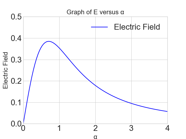
- \(\alpha=0.727\space (Answer)\)
- \(\alpha=0.192\space (Answer)\)
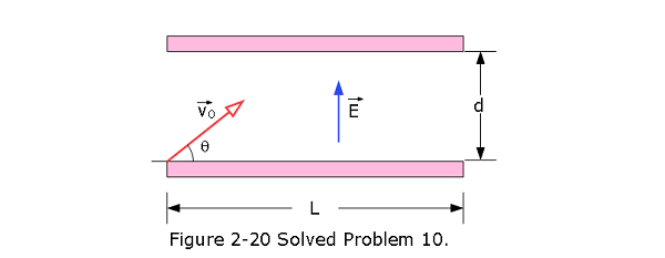
- [84] In Fig. 2-20, a uniform, upward electric field \(\vec E\) of magnitude \(2.00 \times 10^3\) N/C has been set up between two horizontal plates by charging the lower plate positively and the upper plate negatively. The plates have length L = 10.0 cm and separation d = 2.00 cm. An electron is then shot between the plates from the left edge of the lower plate. The initial velocity \(\vec v_0\) of the electron makes an angle \(\theta_0 = 45^\circ\) with the lower plate and has a magnitude of \(6.00 \times 10^6\) m/s. (a) Will the electron strike one of the plates? (b) If so, which plate and how far horizontally from the left edge will the electron strike?
Solution:
- This is a projectile motion, the x equation remains unchanged but the y-equation is a parabolic equation that changes.
\[x = (v_0\cos\theta_0)t\] \[v_x = (v_0\cos\theta_0)\] \[y = (v_0\sin\theta_0)t-\frac{1}{2}at^2\] \[v_y = (v_0\sin\theta_0)-at\] At the maximum height \(v_y = 0\) and the time to reach that height is \(t = \frac{v_0\sin\theta_0}{a}\). Substituting we get the maximum height as \[y_{max}=(v_0\sin\theta_0)\frac{v_0\sin\theta_0}{a}-\frac{1}{2}a\left(\frac{v_0\sin\theta_0}{a}\right)^2\]
Now substituting the acceleration \(a = \frac{eE}{m}\) \[y_{max}=\frac{m}{2}\frac{v_0^2\sin\theta_0^2}{eE}=\frac{(9.1\times 10^{-31}\space kg)(6.00 \times 10^6\space m/s)^2 (\sin45^\circ)^2}{2(1.6 \times 10^{-19}\space C)(2.00 \times 10^3\space N/C)} = 2.56\space cm\gt d\] Therefore, the electron will strike the upper plate. (b) To calculate how far horizontally from the left edge will the electron strike, we need to find x using \(x = (v_0\cos\theta_0)t\). But we need the time it takes to strike the upper plate that can be calculated by setting \(y = d\). Thus,
\[y = d = (v_0\sin\theta_0)t-\frac{1}{2}at^2\] \[\frac{1}{2}at^2 - (v_0\sin\theta_0)t + d =0\] However, it is a quadratic equation with two roots, taking the accetable root, we get
\[t= \frac{v_0sin\theta_0\pm \sqrt{(v_0sin\theta_0)^2-4\times (1/2)ad}}{2\times (1/2)a}=\frac{v_0sin\theta_0\pm \sqrt{v_0^2sin\theta_0^2-2ad}}{a}\] Using \(a = \frac{eE}{m}=\frac{(1.6\times 10^{-19}\space C)(2.00 \times 10^3\space N/C)}{9.1\times 10^{-31}\space kg}=3.51\times 10^{14}\space m/s^2\) \[t= \frac{(6.00 \times 10^6\space m/s) (\sin45^\circ)\pm \sqrt{(6.00 \times 10^6\space m/s)^2 (\sin45^\circ)^2-2(3.51\times 10^{14}\space m/s^2)(2\space m)}}{3.51\times 10^{14}\space m/s^2}\] \[t= \frac{4.24 \times 10^{-8}\space m/s\pm 1.99 \times 10^{-8}\space m/s}{3.51}=4.81\times 10^{-8}\space s, 0.64\times 10^{-8} \space s\] Realistically, the smaller time is the time when electron strikes the upper plate, thus
\[x = (v_0\cos\theta_0)t=(6.00 \times 10^6\space m/s) (\cos45^\circ)(0.64\times 10^{-8}\space s)=2.72\times 10^{-2}\space m=2.72\space cm\space (Answer)\] Using the other we get \(x = 20.41\space cm\space\) which is much longer the length of the plate \(L = 10.0 cm\) and is unacceptable.
Problems Electric Fields
Section 2-1 The Electric Field
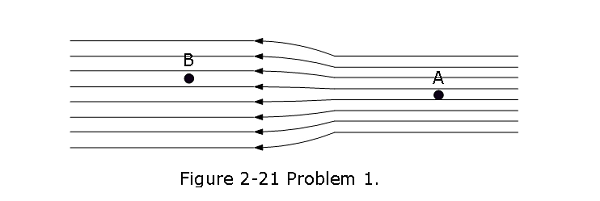
- [2] In Fig. 2-21 the electric field lines on the left have twice the separation of those on the right. (a) If the magnitude of the field at A is 40 N/C, what is the magnitude of the force on a proton at A?(b) What is the magnitude of the field at B?
Section 2-2 The Electric Field Due to a Charged Particle
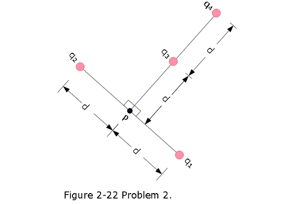
- [8] In Fig. 2-22, the four particles are fixed in place and have charges \(q_1 = q_2 = +5e\), \(q_3 = +3e\), and \(q_4 = -12e\). Distance d = 5.0 \(\mu m\).What is the magnitude of the net electric field at point P due to the particles?
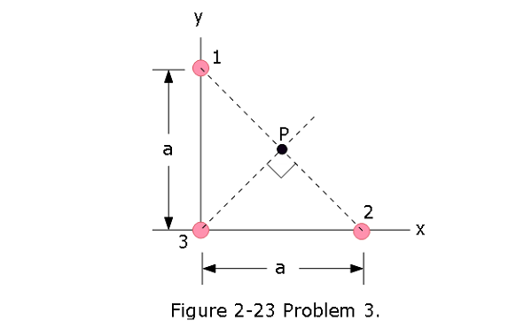
- [15] In Fig. 2-23, the three particles are fixed in place and have charges \(q_1 = q_2 = +e\) and \(q_3 = +2e\). Distance a = 6.00 \(\mu m\). What are the (a) magnitude and (b) direction of the net electric field at point P due to the particles?
Section 2-3 The Electric Field Due to a Dipole
- [18] The electric field of an electric dipole along the dipole axis is approximated by Eqs. 22-8 and 22-9. If a binomial expansion is made of Eq. 22-7, what is the next term in the expression for the dipole’s electric field along the dipole axis? That is, what is \(E_{next}\) in the expression
\[E = \frac{1}{2\pi\varepsilon_{0}}\frac{qd}{z^3}+E_{next}?\]
- [20] Equations 2-10 and 2-11 are approximations of the magnitude of the electric field of an electric dipole, at points along the dipole axis. Consider a point P on that axis at distance z = 5.00d from the dipole center (d is the separation distance between the particles of the dipole). Let \(E_{appr}\) be the magnitude of the field at point P as approximated by Eqs. 2-10 and 2-11. Let \(E_{act}\) be the actual magnitude. What is the ratio \(E_{appr}/E_{act}\)?
Section 2-4 The Electric Field Due to a Line of Charge
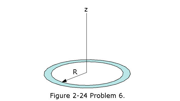
- [24] A thin nonconducting rod with a uniform distribution of positive charge Q is bent into a complete circle of radius R (Fig. 2-24). The central perpendicular axis through the ring is a z axis, with the origin at the center of the ring. What is the magnitude of the electric field due to the rod at (a) z = 0 and (b) \(z = \infty\)? (c) In terms of R, at what positive value of z is that magnitude maximum? (d) If R = 2.00 cm and Q = 4.00 \(\mu C\), what is the maximum magnitude?
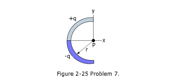
- [26] In Fig. 2-25, a thin glass rod forms a semicircle of radius r = 5.00 cm. Charge is uniformly distributed along the rod, with +q = 4.50 pC in the upper half and -q = -4.50 pC in the lower half. What are the (a) magnitude and (b) direction (relative to the positive direction of the x axis) of the electric field at P, the center of the semicircle?
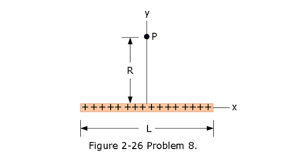
- [32] In Fig. 2-26, positive charge q ! 7.81 pC is spread uniformly along a thin nonconducting rod of length L = 14.5 cm. What are the (a) magnitude and (b) direction (relative to the positive direction of the x axis) of the electric field produced at point P, at distance R = 6.00 cm from the rod along its perpendicular bisector?
Section 2-5 The Electric Field Due to a Charged Disk
[34] A disk of radius 2.5 cm has a surface charge density of 5.3 \(\mu C/m^2\) on its upper face.What is the magnitude of the electric field produced by the disk at a point on its central axis at distance z = 12 cm from the disk?
[35] At what distance along the central perpendicular axis of a uniformly charged plastic disk of radius 0.600 m is the magnitude of the electric field equal to one-half the magnitude of the field at the center of the surface of the disk?
Section 2-6 A Point Charge in an Electric Field
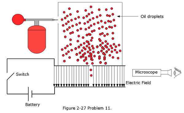
- [39] In Millikan’s experiment, an oil drop of radius 1.64 mm and density 0.851 \(g/cm^3\) is suspended in chamber C (Fig. 2-27) when a downward electric field of \(1.92 \times 10^5\) N/C is applied. Find the charge on the drop, in terms of e.
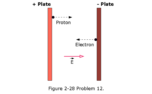
- [53] Two large parallel copper plates are 5.0 cm apart and have a uniform electric field between them as depicted in Fig. 2-28. An electron is released from the negative plate at the same time that a proton is released from the positive plate. Neglect the force of the particles on each other and find their distance from the positive plate when they pass each other. (Does it surprise you that you need not know the electric field to solve this problem?)
Section 2-7 A Dipole in an Electric Field
[56] An electric dipole consists of charges +2e and -2e separated by 0.78 nm. It is in an electric field of strength \(3.4 \times 10^6\) N/C. Calculate the magnitude of the torque on the dipole when the dipole moment is (a) parallel to, (b) perpendicular to, and (c) antiparallel to the electric field.
[57] An electric dipole consisting of charges of magnitude 1.50 nC separated by 6.20 \(\mu m\) is in an electric field of strength 1100 N/C.What are (a) the magnitude of the electric dipole moment and (b) the difference between the potential energies for dipole orientations parallel and antiparallel to \(\vec E\)?