Chapter 10 Induction and Inductance

Learning Objectives:

In this chapter you will basically learn:

$\bullet$ The number of magnetic field piercing a surface is the magnetic flux $\Phi$ through the surface.

$\bullet$ An area vector for a flat surface is a vector that is perpendicular to the surface and that has a magnitude equal to the area of the surface.

$\bullet$ Calculate the magnetic flux $\Phi$ through a surface by integrating the dot product of the magnetic field vector $\vec B$ and the area vector $d\vec A$ (for patch elements) over the surface, in magnitude-angle notation and unit-vector notation.

$\bullet$ Apply Faraday’s law, which is the relationship between an induced emf in a conducting loop and the rate at which magnetic flux through the loop changes.

$\bullet$ Use a right-hand rule for Lenz’s law to determine the direction of induced emf and induced current in a conducting loop.

$\bullet$ Identify that when a magnetic flux through a loop changes, the induced current in the loop sets up a magnetic field to oppose that change.

$\bullet$ If an emf is induced in a conducting loop containing a battery, determine the net emf and calculate the corresponding current in the loop.

$\bullet$ For a conducting loop pulled into or out of a magnetic field, calculate the rate at which energy is transferred to thermal energy.

$\bullet$ Describe eddy currents.

$\bullet$ Identify that a changing magnetic field induces an electric field, regardless of whether there is a conducting loop.

$\bullet$ Apply Faraday’s law to relate the electric field $\vec E$ induced along a closed path (whether it has conducting material or not) to the rate of change $\frac{d\Phi}{dt}$ of the magnetic flux encircled by the path.

$\bullet$ For an inductor, apply the relationship between inductance L, total flux $N\Phi$, and current i.

$\bullet$ For a solenoid, apply the relationship between the inductance per unit length $L/l$, the area A of each turn, and the number of turns per unit length n.

$\bullet$ Apply the relationship between the induced emf in a coil, the coil’s inductance L, and the rate di/dt at which the current is changing.

$\bullet$ When an emf is induced in a coil because the current in the coil is changing, determine the direction of the emf by using Lenz’s law to show that the emf always opposes the change in the current, attempting to maintain the initial current.

$\bullet$ For an RL circuit in which the current is rising, find equations for the potential difference V across the resistor, the rate di/dt at which the current changes, and the emf of the inductor, as functions of time.

$\bullet$ Calculate an inductive time constant $\tau_L$.

$\bullet$ Write a loop equation (a differential equation) for an RL circuit in which the current is decaying.

$\bullet$ For an RL circuit in which the current is decaying, apply the equation i(t) for the current as a function of time.

$\bullet$ From an equation for decaying current in an RL circuit, find equations for the potential difference V across the resistor, the rate di/dt at which current is changing, and the emf of the inductor, as functions of time.

$\bullet$ For an RL circuit, identify the current through the inductor and the emf across it just as current in the circuit begins to change (the initial condition) and a long time later when equilibrium is reached (the final condition).

$\bullet$ Describe the derivation of the equation for the magnetic field energy of an inductor in an RL circuit with a constant emf source.

$\bullet$ For an inductor in an RL circuit, apply the relationship between the magnetic field energy U, the inductance L, and the current i.

$\bullet$ Identify that energy is associated with any magnetic field.

$\bullet$ Apply the relationship between energy density $u_B$ of a magnetic field and the magnetic field magnitude B.

$\bullet$ Calculate the mutual inductance of one coil with respect to a second coil (or some second current that is changing).

$\bullet$ Calculate the emf induced in one coil by a second coil in terms of the mutual inductance and the rate of change of the current in the second coil.

10.1 Induction and Inductance:

10.2 Faraday’s Law of Induction:

Similar to electric flux we defined in Eq 3-1$\Phi_E = \oint {\vec E.d\vec A}$,we need to define a magnetic flux. Suppose a loop enclosing an area A is placed in a magnetic field $\vec B$.Then the magnetic flux through the loop is

\[\begin{equation} \Phi_B = \int \vec B.d\vec A ~~~(magnetic~flux~through~area~A). \tag{10.1} \end{equation}\]

As a special case of Eq. 10-1, suppose that the loop lies in a plane and that the magnetic field is perpendicular to the plane of the loop. Then we can write the dot product in Eq. 10-1 as $B~dA~cos0^0 = B~dA$. If the magnetic field is also uniform, then B can be taken outside the integral sign. The remaining $\int dA$ then gives just the area A of the loop. Thus, Eq. 10-1 reduces to

\[\begin{equation} \Phi_B = BA ~~~(magnetic~flux~through~area~A). \tag{10.2} \end{equation}\]

SI Unit of Flux: From Eqs. 10-1 and 10-2,we see that the SI unit for magnetic flux is the tesla–square meter, which is called the weber (abbreviated Wb):

\[\begin{equation} 1 weber = 1 Wb = 1~T.m^2 \tag{10.3} \end{equation}\]

The magnitude of the emf $\varepsilon$ induced in a conducting loop is equal to the rate at which the magnetic flux $\Phi_B$ through that loop changes with time is known as Faraday’s law of induction. The induced emf $\varepsilon$ tends to oppose the flux change, as can be seen in the formal equation of Faraday’s law with a negative sign:

\[\begin{equation} \mathcal{E} = -\frac{d\Phi_B}{dt}~~~(Faraday’s~law), \tag{10.4} \end{equation}\]

We normally neglect the minus sign in Eq. 10-4, and use only the magnitude of the induced emf.

For a tightly packed coil with N number of turns, Faraday’s can be modified to

\[\begin{equation} \mathcal{E} = -N\frac{d\Phi_B}{dt}~~~(Faraday’s~law~for~N~turns), \tag{10.5} \end{equation}\]

10.3 Lenz’s Law:

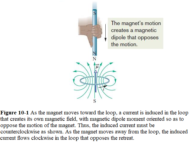
An induced current has a direction such that the magnetic field due to the current opposes the change in the magnetic flux that induces the current. The key word in Lenz’s law is “opposition.”

As the north pole of the magnet gets closer to the loop as in Fig. 10-1, the magnetic flux increases through the loop and thereby induces a current in the loop. In Fig. 9-10, we know that the loop then acts as a magnetic dipole with a south pole and a north pole, and that its magnetic dipole moment is directed from south to north. To oppose the magnetic flux increase being caused by the approaching magnet, the loop’s north pole (and thus ) must face toward the approaching north pole so as to repel it (Fig. 10-1). Then the curled – straight right-hand rule for (Fig. 9-10) tells us that the current induced in the loop must be counterclockwise in Fig. 10-1. If we next pull the magnet away from the loop, a current will again be induced in the loop. Now, however, the loop will have a south pole facing the retreating north pole of the magnet, so as to oppose the retreat. Thus, the induced current will be clockwise.

10.4 Induction and Energy Transfers:

By Lenz’s law, whether you move the magnet toward or away from the loop in Fig. 10-1, a magnetic force resists the motion, requiring your applied force to do positive work. At the same time, thermal energy is produced in the material of the loop because of the material’s electrical resistance to the current that is induced by the motion.The energy you transfer to the closed loop & magnet system via your applied force ends up in this thermal energy. (For now, we neglect energy that is radiated away from the loop as electromagnetic waves during the induction.) The faster you move the magnet, the more rapidly your applied force does work and the greater the rate at which your energy is transferred to thermal energy in the loop; that is, the power of the transfer is greater.

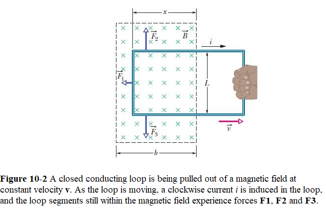
Rate of Work. As you will see, to pull the loop at a constant velocity , you must apply a constant force to the loop because a magnetic force of equal magnitude but opposite direction acts on the loop to oppose you. The rate at which you do work—that is, the power—is then

\[\begin{equation} P = Fv \tag{6.11} \end{equation}\]

where F is the magnitude of the force. An expression for P in terms of the magnitude B of the magnetic field and its resistance R to current and its dimension L. As you move the loop to the right in Fig. 10-2, the portion of its area within the magnetic field decreases. Thus, the flux through the loop also decreases and, according to Faraday’s law, a current is produced in the loop. It is the presence of this current that causes the force that opposes the pull.

Induced emf. To find the current, we first apply Faraday’s law. When x is the length of the loop still in the magnetic field, the area of the loop still in the field is Lx.Then from Eq. 10-2, the magnitude of the flux through the loop is

\[\begin{equation} \Phi_B = BA = BLx \tag{10.6} \end{equation}\]

Ignoring the minus sign in Faraday’s law in Eq. 10-4 and using Eq. 10-7, we can write the magnitude of this emf as

\[\begin{equation} \mathcal{E} = \frac{d\Phi_B}{dt}=\frac{d}{dt}BLx=BL\frac{dx}{dt}=BLv \tag{7.1} \end{equation}\]

in which we have replaced $dx/dt$ with v, the speed at which the loop moves.

Induced Current. We can use the equation $i=\varepsilon/R$ in Eq. 10-8, it becomes

\[\begin{equation} i = \frac{BLv}{R} \tag{10.7} \end{equation}\]

We can find the magnitude of $\vec F_1$ and by considering the angle between $\vec B$ and the length vector $\vec L$ for the left segment is $90^0$, we write

\[\begin{equation} F = F_1 = iLB~\sin90^0=iLB \tag{10.8} \end{equation}\]

Substituting Eq. 10-9 for i in Eq. 10-10 then gives us

\[\begin{equation} F = \frac{B^2L^2v}{R} \tag{10.9} \end{equation}\]

Because B, L, and R are constants, the speed v at which you move the loop is constant if the magnitude F of the force you apply to the loop is also constant.

Rate of Work. By substituting Eq. 10-11 into Eq. 10-6, we find the rate at which you do work on the loop as you pull it from the magnetic field:

\[\begin{equation} P = Fv = \frac{B^2L^2v^2}{R}~~~(rate~of~doing~work). \tag{6.12} \end{equation}\]

Thermal Energy. The rate at which thermal energy appears in the loop is

\[\begin{equation} P = i^2R = \left(\frac{BLv}{R}\right)^2R=\frac{B^2L^2v^2}{R} ~~~(thermal~energy~rate). \tag{6.13} \end{equation}\]

which is exactly equal to the rate at which you are doing work on the loop (Eq. 10-12).Thus, the work that you do in pulling the loop through the magnetic field appears as thermal energy in the loop.

10.5 Induced Electric Fields:

A changing magnetic field produces an electric field.

\[\begin{equation} \mathcal{E} = \oint \vec E.d\vec s \tag{10.10} \end{equation}\]

Combining Eq. 10-14 with Faraday’s law in Eq. 10-4, we can rewrite Faraday’s law as

\[\begin{equation} \oint \vec E.d\vec s = -\frac{d\Phi_B}{dt}~~~(Faraday’s~law), \tag{10.11} \end{equation}\]

The potential difference between two points i and f in an electric field $\vec E$ in terms of an integration between those points:

\[\begin{equation} V_f-V_i = -\int_{i}^{f} \vec E.d\vec s \tag{4.4} \end{equation}\]

If i and f in Eq. 10-16 are the same point, the path connecting them is a closed loop, $V_i$ and $V_f$ are identical, and Eq. 10-16 reduces to

\[\begin{equation} \int_{i}^{f} \vec E.d\vec s = 0 \tag{4.11} \end{equation}\]

However, when a changing magnetic flux is present, this integral is not zero but is $- $, as Eq. 10-15 asserts. Thus, assigning electric potential to an induced electric field leads us to a contradiction.We must conclude that electric potential has no meaning for electric fields associated with induction.

10.6 Inductors and Inductance:

The inductance of the inductor is then defined in terms of that flux as

\[\begin{equation} L = \frac{N\Phi_B}{i}~~~(inductance), \tag{10.12} \end{equation}\]

where N is the number of turns. The windings of the inductor are said to be linked by the shared flux, and the product $N\Phi_B$ is called the magnetic flux linkage. The inductance L is thus a measure of the flux linkage produced by the inductor per unit of current.

Because the SI unit of magnetic flux is the tesla–square meter, the SI unit of inductance is the tesla–square meter per ampere $\frac{T-m^2}{A}$. We call this the henry (H), after American physicist Joseph Henry, the codiscoverer of the law of induction and a contemporary of Faraday.Thus,

\[\begin{equation} 1~henry=1~H=1~\frac{T-m^2}{A} \tag{10.13} \end{equation}\]

10.7 Inductance of a Solenoid:

Consider a long solenoid of cross-sectional area A as we discussed in Section 9-5. To find the inductance per unit length of a solenoid we make use of equation for inductance (Eq. 10-18), and the equation for magnetic field in Eq. 9-19 set up by a given current in the solenoid windings. Consider a length l near the middle of this solenoid, by substituting the flux linkage as given by $N\Phi_B=(nl)(BA)$ in Eq. 10-18 and using magnetic field as given in Eq. 9-19, we get the inductance per unit length near the center of a long solenoid as follows:

\[L = \frac{N\Phi_B}{i}~~~(inductance)~~~(Eq. 10-18)\] \[B = \mu_0 in~~~(ideal~solenoid)~~~(Eq. 9-19)\]

\[\begin{equation} \frac{L}{l}=\mu_0n^2A~~~(solenoid) \tag{10.14} \end{equation}\]

Inductance—like capacitance ($C=\frac{\epsilon_0A}{d}$)—depends only on the geometry of the device. The dependence on the square of the number of turns per unit length is to be expected.

The permeability constant $\mu_0$ and a quantity with the dimensions of a length. This means that $\mu_0$ can be expressed in the unit henry per meter:

\[\begin{equation} \mu_0 = 4\pi \times 10^{-7}~~ \frac{T.m}{A}=4\pi\times 10^{-7}~~\frac{H}{m} \tag{10.15} \end{equation}\]

10.8 Self-Induction:

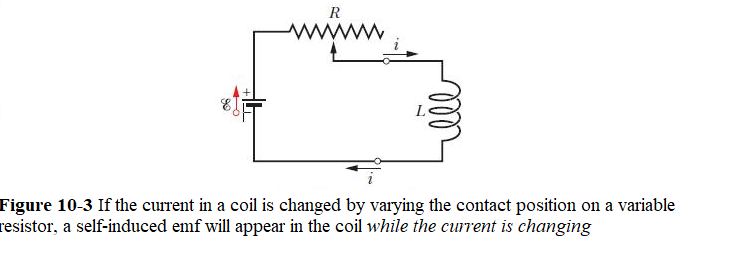
If a current i in a coil changes with time, an emf is induced in the coil. This self-induced emf appears in any coil in which the current is changing. This process (see Fig. 10-3) is called self-induction, and the emf that appears is called a self-induced emf. It obeys Faraday’s law of induction just as other induced emfs do. For any inductor, Eq. 10-18 tells us that

\[\begin{equation} Li = N\Phi_B \tag{10.16} \end{equation}\]

Using Faraday’s law we get

\[\begin{equation} \mathcal{E_L} = -\frac{dN\Phi_B}{dt}=-L\frac{di}{dt} \tag{10.17} \end{equation}\]

Thus, in any inductor (such as a coil, a solenoid, or a toroid) a self-induced emf appears whenever the current changes with time. The magnitude of the current has no influence on the magnitude of the induced emf; only the rate of change of the current counts.

10.9 RL Circuits:

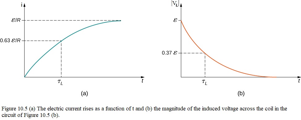
If a constant emf is introduced into a single-loop circuit containing a resistance R and an inductance L, the current rises to an equilibrium value of $\mathcal{E}/R$ according to \[i=\frac{\mathcal{E}}{R}(1-e^{-t/\tau_L})~~~(rise~of~current).\]

Applying Kirchhoff’s loop rule to this circuit in Fig. 10-4, we obtain

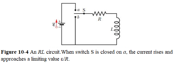
\[\begin{equation} \mathcal{E}-L\frac{di}{dt}-iR=0 \tag{10.18} \end{equation}\]

\[\frac{di}{dt}=\frac{\mathcal{E}}{L}-\frac{iR}{L}=\frac{\mathcal{E}-iR}{L}\] \[\int \frac{di}{\mathcal{E}-iR}=\frac{1}{L}\int dt\] Let’s assume $u=\mathcal{E-iR}, du=-Rdi$, we get \[\int_0^{i}\frac{du}{u}=-\frac{R}{L}\int_0^{t}dt\] \[\ln~u|_0^{i}=-\frac{Rt}{L}|_0^{t}\] \[\ln(\mathcal{E}-iR)-ln\mathcal{E}=-\frac{Rt}{L}\] \[\frac{\mathcal{E}-iR}{\mathcal{E}}=e^{-Rt/L}=e^{-t/\tau_L}\] where $\tau_L=\frac{L}{R}$ is called the inductive time constant.

\[\begin{equation} i=\frac{\mathcal{E}}{R}\left(1-e^{-\frac{t}{\tau_L}}\right)~~~(rise~of~current). \tag{10.19} \end{equation}\]

The current i(t) is plotted in Figure 10.5(a). It starts at zero, and as $t\rightarrow\infty$, i(t) approaches asymptotically to $\mathcal{E}/R$. The induced emf $\mathcal{E}_L(t)$ is directly proportional to di/dt, or the slope of the curve. Therefore, it starts from its maximum value Figure 10.5(b) after the switch is thrown to a, the induced emf decreases to zero with time as the current approaches its final value of $\mathcal{E}/R$. The circuit then becomes equivalent to a resistor connected across a source of emf.

We can also see how the potential differences across the resistor and inductor happens as time increases in Fig. 10-6. The potential differences $(V_R = iR)$ across the resistor and $V_L (= L di/dt)$ across the inductor vary with time for particular values of $\mathcal{E}$, L, and R. Compare this figure carefully with the corresponding figure for an RC circuit (Fig. 7-12).

The quantity $\tau_L (= L/R)$ in the exponential of Eq. 10-25 has the dimension of time because the argument of the exponential function in Eq. 10-25 must have to be dimensionless), that we can show as follows:

\[\tau_L=\frac{L}{R}=\frac{\tau_Ldt/di}{V/i}=\frac{V.s.A}{A.V}=1~s\] The differential equation that governs the decay can be found by disconnecting the battery () in Eq. 10-24:

\[\begin{equation} L\frac{di}{dt}+ iR=0 \tag{10.20} \end{equation}\]

The solution to Eq.10-26 that satisfies the initial condition $i(0)=i_0=\frac{\mathcal{E}}{R}$ is

\[\begin{equation} i=\frac{\mathcal{E}}{R}e^{-\frac{t}{\tau_L}}=i_0e^{-\frac{t}{\tau_L}} ~~~(decay~of~current). \tag{10.21} \end{equation}\]

10.10 Energy Stored in a Magnetic Field:

If we multiply each side of Eq. 10-24 by i,we obtain

\[\mathcal{Ei}-Li\frac{di}{dt}-i^2R=0\]

\[\frac{dU_B}{dt}=Li\frac{di}{dt}\] \[\int_0^{U_B}dU_B=\int_0^{i}Lidt\]

\[\begin{equation} U_B=\frac{1}{2}Li^2~~~(magnetic~energy) \tag{10.22} \end{equation}\]

Comparing to Eq.10-28, to the electric energy we found in Eq. 5-21 ($U_E = \frac{q^2}{2C}=\frac{1}{2}CV^2$)

10.11 Energy Density of a Magnetic Field:

Energy density of a magnetic field is defined to be the energy stored per unit volume of the field is

\[u_B=\frac{U_B}{Al}\] using the result of Eq. 10-28 $U_B=\frac{1}{2}Li^2$, we get

\[\begin{equation} u_B=\frac{Li^2}{2Al}=\left(\frac{L}{l}\right)\frac{i^2}{2A} \tag{10.23} \end{equation}\]

Now substituting for $ from Eq. 10-20, we get

\[\begin{equation} u_B=\frac{1}{2l}\mu_0n^2i^2 \tag{10.24} \end{equation}\]

where n is the number of turns per unit length. From Eq. 9-19 $(B = \mu_0in)$ we can get the magnetic energy density as

\[\begin{equation} u_B=\frac{B^2}{2\mu_0l}~~~(magnetic ~energy ~density). \tag{10.25} \end{equation}\]

A similar equation for electric energy density was discussed in Eq. 5-22,

\[\begin{equation} u_E=\frac{1}{2}\epsilon_0E^2~~~(magnetic ~energy ~density). \tag{5.22} \end{equation}\]

which gives the energy density (in a vacuum) at any point in an electric field. One thing we can see that both $u_B$ and $u_E$ are proportional to the square of the appropriate field magnitude, B or E.

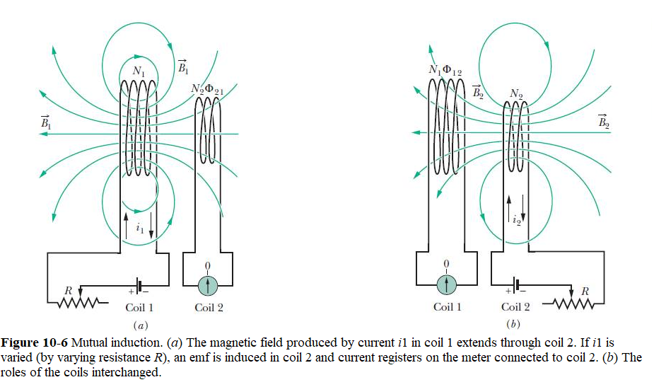
10.12 Mutual Induction:

We define the mutual inductance $M_{21}$ of coil 2 with respect to coil 1 as

\[\begin{equation} M_{21}=\frac{N_2\Phi_{21}}{i_1} \tag{10.26} \end{equation}\]

which has the same form as Eq. 10-18, $L = \frac{N\Phi_B}{i}$. Comparing Eq. 10-33 with Eq. 10-18, we can easily see that inductance, L is replaced by mutual-inductance, M in Eq. 10-33.

Considering the time derivative of $i_1$ by varying R, we have

\[\begin{equation} M_{21}\frac{di_1}{dt}=N_2\frac{d\Phi_{21}}{dt} \tag{10.27} \end{equation}\]

The right side of this equation (Eq. 10-34) is, according to Faraday’s law, just the magnitude of the emf $\mathcal{E_2}$ appearing in coil 2 due to the changing current in coil 1. Thus, with a minus sign to indicate direction,

\[\begin{equation} \mathcal{E_2}=-M_{21}\frac{di_1}{dt} \tag{10.28} \end{equation}\]

Eq. 10-35 is comparable to self-induction ($\mathcal{E}=-L\frac{di}{dt}$).

By interchanging the roles of coils 1 and 2, as in Fig. 10-6b; that is, we set up a current $i_2$ in coil 2 by means of a battery, and this produces a magnetic flux $\Phi_{12}$ that links coil 1. Similarly, by varying $i_2$ with time by varying R, we then get,

\[\begin{equation} \mathcal{E_1}=-M_{12}\frac{di_2}{dt} \tag{10.29} \end{equation}\]

Assuming without proof,

\[\begin{equation} M_{21}=M_{12}=M \tag{10.30} \end{equation}\]

Finally, we get the equations for mutual inductances.

\[\begin{equation} \mathcal{E_2}=-M\frac{di_1}{dt} \tag{10.31} \end{equation}\]

and

\[\begin{equation} \mathcal{E_1}=-M\frac{di_2}{dt} \tag{10.32} \end{equation}\]

Solved Problems Induction and Inductance

[3] In Fig. 30-34, a 120-turn coil of radius 1.8 cm and resistance 5.3 $\Omega$ is coaxial with a solenoid of 220 turns/cm and diameter 3.2 cm. The solenoid current drops from 1.5 A to zero in time interval $\Delta t$ = 25 ms. What current is induced in the coil during $\Delta t$?
[7] In Fig. 30-38, the magnetic flux ! (4.00 $ through the loop increases according to the relation $\Phi_B = 6.0t^2 + 7.0t$, where $\Phi_B$ is in milliwebers and t is in seconds. (a) What is the magnitude of the emf induced in the loop when t = 2.0 s? (b) Is the direction of the current through R to the right or left?
[11] A rectangular coil of N turns and of length a and width b is rotated at frequency f in a uniform magnetic field $\vec B$, as indicated in Fig. 30-40. The coil is connected to co-rotating cylinders, against which metal brushes slide to make contact. (a) Show that the emf induced in the coil is given (as a function of time t) by

$\mathcal{E} = 2\pi fNabB\sin(2\pi ft)=\mathcal{E}_0sin(2\pi ft)$.

This is the principle of the commercial alternating-current generator. (b) What value of Nab gives an emf with $\mathcal{E}_0$ = 150 V when the loop is rotated at 60.0 rev/s in a uniform magnetic field of 0.500 T?

[12] In Fig. 30-41, a wire loop of lengths L = 40.0 cm and W = 25.0 cm lies in a magnetic field $\vec B$. What are the (a) magnitude and (b) direction (clockwise or counterclockwise—or “none” if $\mathcal{E}$ = 0) of the emf induced in the loop if $\vec B = (4.00\times 10^{-2}~T/m)y\hat k$? What are (c) $\mathcal {E}$ and (d) the direction if $\vec B = (6.00\times 10^{-2}~T/s)t\hat k$? What are (e) $\mathcal {E}$ and (f) the direction if $\vec B = (8.00\times 10^{-2}~T/m.s)yt\hat k$? What are (g) $\mathcal {E}$ and (h) the direction if $\vec B = (8.00\times 10^{-2}~T/m.s)xt\hat j$? What are (i) $\mathcal {E}$ and (j) the direction if $\vec B = (8.00\times 10^{-2}~T/m.s)yt\hat i$?
[15] A square wire loop with 2.00 m sides is perpendicular to a uniform magnetic field, with half the area of the loop in the field as shown in Fig. 30-43. The loop contains an ideal battery with emf $\mathcal {E}$ = 20.0 V. If the magnitude of the field varies with time according to B = 0.0420 - 0.870t, with B in teslas and t in seconds, what are (a) the net emf in the circuit and (b) the direction of the (net) current around the loop?
[26] For the wire arrangement in Fig. 30-49, a 12.0 cm and b 16.0 cm. The current in the long straight wire is $i = 4.50t^2 - 10.0t$, where i is in amperes and t is in seconds. (a) Find the emf in the square loop at t = 3.00 s. (b) What is the direction of the induced current in the loop?
[29] In Fig. 30-52, a metal rod is forced to move with constant velocity along two parallel metal rails, connected with a strip of metal at one end. A magnetic field of magnitude B = 0.350 T points out of the page. (a) If the rails are separated by L = 25.0 cm and the speed of the rod is 55.0 cm/s, what emf is generated? (b) If the rod has a resistance of 18.0 $\Omega$ and the rails and connector have negligible resistance, what is the current in the rod? (c) At what rate is energy being transferred to thermal energy?
[33] Figure 30-54 shows a rod of length L = 10.0 cm that is forced to move at constant speed v = 5.00 m/s along horizontal rails. The rod, rails, and connecting strip at the right form a conducting loop. The rod has resistance 0.400 $\Omega$; the rest of the loop has negligible resistance. A current i = 100 A through the long straight wire at distance a = 10.0 mm from the loop sets up a (nonuniform) magnetic field through the loop. Find the (a) emf and (b) current induced in the loop. (c) At what rate is thermal energy generated in the rod? (d) What is the magnitude of the force that must be applied to the rod to make it move at constant speed? (e) At what rate does this force do work on the rod?
[36] Figure 30-56 shows two circular regions $R_1$ and $R_2$ with radii $r_1$ = 20.0 cm and $r_2$ = 30.0 cm. In $R_1$ there is a uniform magnetic field of magnitude $B_1$ = 50.0 mT directed into the page, and in $R_2$ there is a uniform magnetic field of magnitude $B_2$ = 75.0 mT directed out of the page (ignore fringing). Both fields are decreasing at the rate of 8.50 mT/s. Calculate $\oint \vec E.d\vec s$ for (a) path 1, (b) path 2, and (c) path 3.
[41] A circular coil has a 10.0 cm radius and consists of 30.0 closely wound turns of wire. An externally produced magnetic field of magnitude 2.60 mT is perpendicular to the coil. (a) If no current is in the coil, what magnetic flux links its turns? (b)When the current in the coil is 3.80 A in a certain direction, the net flux through the coil is found to vanish.What is the inductance of the coil?
[45] At a given instant the current and self-induced emf in an inductor are directed as indicated in Fig. 30-59. (a) Is the current increasing or decreasing? (b) The induced emf is 17 V, and the rate of change of the current is 25 kA/s; find the inductance.
[47] Inductors in series. Two inductors $L_1$ and $L_2$ are connected in series and are separated by a large distance so that the magnetic field of one cannot affect the other. (a) Show that the equivalent inductance is given by \[L_{eq} = L_1 + L_2\].
[48] Inductors in parallel. Two inductors $L_1$ and $L_2$ are connected in parallel and separated by a large distance so that the magnetic field of one cannot affect the other. (a) Show that the equivalent inductance is given by \[\frac{1}{L_{eq}} = \frac{1}{L_1} + \frac{1}{L_2}\].
[54] In Fig. 30-62, $\mathcal{E}$ = 100 V, $R_1$ = 10.0 $\Omega$, $R_2$ = 20.0 $\Omega$, $R_3$ = 30.0 $\Omega$, and L = 2.00 H. Immediately after switch S is closed, what are (a) $i_1$ and (b) $i_2$? (Let currents in the indicated directions have positive values and currents in the opposite directions have negative values.) A long time later, what are (c) $i_1$ and (d) $i_2$? The switch is then reopened. Just then, what are (e) $i_1$ and (f) $i_2$? A long time later, what are (g) $i_1$ and (h) $i_2$?
[62] A coil with an inductance of 2.0 H and a resistance of 10 ” is suddenly connected to an ideal battery with $\mathcal{E}$ = 100 V. At 0.10 s after the connection is made, what is the rate at which (a) energy is being stored in the magnetic field, (b) thermal energy is appearing in the resistance, and (c) energy is being delivered by the battery?
[66] A circular loop of wire 50 mm in radius carries a current of 100 A. Find the (a) magnetic field strength and (b) energy density at the center of the loop.
[69] What must be the magnitude of a uniform electric field if it is to have the same energy density as that possessed by a 0.50 T magnetic field?
[75] A rectangular loop of N SSM closely packed turns is positioned near a long straight wire as shown in Fig. 30-68. What is the mutual inductance M for the loop–wire combination if N = 100, a = 1.0 cm, b = 8.0 cm, and l = 30 cm?

Problems Induction and Inductance

Section 10-1 Faraday’s Law and Lenz’s Law

[4] A wire loop of radius 12 cm and resistance 8.5 $\Omega$ is located in a uniform magnetic field $\vec B$ that changes in magnitude as given in Fig. 30-35. The vertical axis scale is set by $B_s$ = 0.50 T, and the horizontal axis scale is set by $t_s$ = 6.00 s. The loop’s plane is perpendicular to $\vec B$. What emf is induced in the loop during time intervals (a) 0 to 2.0 s, (b) 2.0 s to 4.0 s, and (c) 4.0 s to 6.0 s?
[14] In Fig. 30-42a, a uniform magnetic field $\vec B$ increases in magnitude with time t as given by Fig. 30-42b, where the vertical axis scale is set by $B_s$ = 9.0 mT and the horizontal scale is set by $t_s$ = 3.0 s. A circular conducting loop of area $8.0 \times 10^4 ~m^2$ lies in the field, in the plane of the page. The amount of charge q passing point A on the loop is given in Fig. 30-42c as a function of t, with the vertical axis scale set by $q_s$ = 6.0 mC and the horizontal axis scale again set by $t_s$ = 3.0 s. What is the loop’s resistance?
[18] In Fig. 30-45, two straight conducting rails form a right angle. A conducting bar in contact with the rails starts at the vertex at time t = 0 and moves with a constant velocity of 5.20 m/s along them. A magnetic field with B = 0.350 T is directed out of the page. Calculate (a) the flux through the triangle formed by the rails and bar at t ! 3.00 s and (b) the emf around the triangle at that time. (c) If the emf is $\mathcal{E} = at^n$, where a and n are constants, what is the value of n?
[21] In Fig. 30-46, a stiff wire bent into a semicircle of radius a = 2.0 cm is rotated at constant angular speed 40 rev/s in a uniform 20 mT magnetic field.What are the (a) frequency and (b) amplitude of the emf induced in the loop?
[28] In Fig. 30-51, a rectangular loop of wire with length a = 2.2 cm, width b = 0.80 cm, and resistance R = 0.40 m$\Omega$ is placed near an infinitely long wire carrying current i = 4.7 A. The loop is then moved away from the wire at constant speed v = 3.2 mm/s. When the center of the loop is at distance r = 1.5b, what are (a) the magnitude of the magnetic flux through the loop and (b) the current induced in the loop?

Section 10-2 Induction and Energy Transfers

[34] In Fig. 30-55, a long rectangular conducting loop, of width L, resistance R, and mass m, is hung in a horizontal, uniform magnetic field $\vec B$ that is directed into the page and that exists only above line aa. The loop is then dropped; during its fall, it accelerates until it reaches a certain terminal speed $v_t$. Ignoring air drag, find an expression for $v_t$.

Section 10-3 Induced Electric Fields

[37] A long solenoid has a diameter of 12.0 cm.When a current i exists in its windings, a uniform magnetic field of magnitude B = 30.0 mT is produced in its interior. By decreasing i, the field is caused to decrease at the rate of 6.50 mT/s. Calculate the magnitude of the induced electric field (a) 2.20 cm and (b) 8.20 cm from the axis of the solenoid.

Section 10-4 Inductors and Inductance

[40] The inductance of a closely packed coil of 400 turns is 8.0 mH. Calculate the magnetic flux through the coil when the current is 5.0 mA.

Section 10-5 Self-Induction

[44] A 12 H inductor carries a current of 2.0 A.At what rate must the current be changed to produce a 60 V emf in the inductor?
[49] The inductor arrangement of Fig. 30-61, with $L_1$ = 30.0 mH, $L_2$ = 50.0 mH, $L_3$ = 20.0 mH, and $L_4$ = 15.0 mH, is to be connected to a varying current source.What is the equivalent inductance of the arrangement? (First see Problems 47 and 48.)

Section 10-6 RL Circuits

[52] The switch in Fig. 30-15 is closed on a at time t = 0. What is the ratio $\frac{\mathcal{E}_L}{\mathcal{E}}$ of the inductor’s self-induced emf to the battery’s emf (a) just after t = 0 and (b) at $t = 2.00\tau_L$? (c) At what multiple of $\tau_L$ will $\frac{\mathcal{E}_L}{\mathcal{E}}=0.500$?
[57] In Fig. 30-65, R = 15 $\Omega$, L = 5.0 H, the ideal battery has $ = $10 V, and the fuse in the upper branch is an ideal 3.0 A fuse. It has zero resistance as long as the current through it remains less than 3.0 A. If the current reaches 3.0 A, the fuse “blows” and thereafter has infinite resistance. Switch S is closed at time t = 0. (a) When does the fuse blow? (Hint: Equation 30-41 does not apply. Rethink Eq. 30-39.) (b) Sketch a graph of the current i through the inductor as a function of time. Mark the time at which the fuse blows.
[59] In Fig. 30-66, after switch S is closed at time t = 0, the emf of the source is automatically adjusted to maintain a constant current i through S. (a) Find the current through the inductor as a function of time. (b) At what time is the current through the resistor equal to the current through the inductor?

Section 10-7 Energy Stored in a Magnetic Field

[64] At t = 0, a battery is connected to a series arrangement of a resistor and an inductor. At what multiple of the inductive time constant will the energy stored in the inductor’s magnetic field be 0.500 its steady-state value?

Section 10-8 Energy Density of a Magnetic Field

[67] A solenoid that is 85.0 cm long has a cross-sectional area of 17.0 $cm^2$. There are 950 turns of wire carrying a current of 6.60 A. (a) Calculate the energy density of the magnetic field inside the solenoid. (b) Find the total energy stored in the magnetic field there (neglect end effects).

Section 10-9 Mutual Induction

[76] A coil C of N turns is placed around a long solenoid S of radius R and n turns per unit length, as in Fig. 30-69. (a) Show that the mutual inductance for the coil–solenoid combination is given by $M = \mu_0\pi R^2nN$. (b) Explain why M does not depend on the shape, size, or possible lack of close packing of the coil.