Lab-8 Window Design

Name: Write down your name

Date: Date of report submission and date of lab performed

Window Design Technique:

As we defined earlier, a causal filter is a linear and time-invariant causal system. The word causal indicates that the filter output depends only on past and present inputs. A filter whose output also depends on future inputs is non-causal, whereas a filter whose output depends only on future inputs is anti-causal. The basic idea behind the window design is to choose a proper ideal frequency-selective filter (which always has a noncausal, infinite-duration impulse response) and then to truncate (to window) its impulse response to obtain a linear-phase and causal FIR filter. Therefore, the emphasis in this method is on selecting an appropriate windowing function and an appropriate ideal filter. We will denote an ideal frequency-selective filter by \(H_d (e^{jω})\), which has a unity magnitude gain and linear-phase characteristics over its passband, and zero response over its stopband. An ideal LPF of bandwidth \(ω_c < π\) is given by

\[\begin{equation} H_d(e^{j\omega})=\begin{cases} 1e^{-j\alpha\omega}, |\omega|\le \omega_c\\ 0, \omega_c\lt|\omega|\le\pi \end{cases} \tag{8.1} \end{equation}\]

where \(ω_c\) is called the cutoff frequency and \(\alpha\) is called the sample delay. (Note that from the DTFT properties, \(e^{-jαω}\) implies shift in the positive n direction or delay.) The impulse response of this filter is of infinite duration and is given by

\[\begin{equation} h_d(n)=\mathcal{F}[H_d(e^{j\omega})]=\frac{1}{2\pi}\int_{-\pi}^{\pi}H_d(e^{j\omega})e^{j\omega n}d\omega=\frac{1}{2\pi}\int_{-\omega_c}^{\omega_c}e^{-j\alpha\omega}e^{j\omega n}d\omega=\frac{sin[\omega_c(n-\alpha)]}{\pi(n-\alpha)} \tag{8.2} \end{equation}\]

Note that \(h_d(n)\) is symmetric with respect to \(\alpha\), a fact useful for linear phase FIR filters.

To obtain an FIR filter from \(h_d (n)\), one has to truncate \(h_d (n)\) on both sides. To obtain a causal and linear-phase FIR filter h(n) of length M, we must have

\[\begin{equation} h(n)=\begin{cases} h_d(n), 0\le n \le M-1, \\ 0, elsewhere \end{cases} \tag{8.3} and\space \alpha = \frac{(M-1)}{2} \end{equation}\]

This operation is called “windowing”. In general, h(n) can be thought of as being formed by the product of h_d (n) and a window function w(n) as follows:

\[\begin{equation} h(n)=h_d(n)w(n) \tag{8.4} \end{equation}\]

where

\[\begin{equation} h(n)=\begin{cases} some\space symmetric\space function\space with\space respect\space to\space \alpha \space over \space 0 \le n \le M-1 \\ 0, otherwise \end{cases} \end{equation}\]

Depending on how we define w(n), we obtain different window designs. For example, in (8.3)

\[\begin{equation} h(n)=\begin{cases} 1,\space 0 \le n \le M-1 \\ 0,elsewhere \end{cases} =\mathcal{R_M(n)} \end{equation}\]

where \(R_M(n)\) is the rectangular window.

In the frequency domain, the causal FIR filter response \(H(e^{j\omega})\) is given by periodic convolution of \(H_d(e^{j\omega})\) and the window response \(W(e^{j\omega})\) that is,

\[\begin{equation} H(e^{j\omega})= H_d (e^{j\omega})\odot W(e^{j\omega})=\frac{1}{2\pi}\int_{-\pi}^\pi W(e^{j\lambda})H_d(e^{j(\omega-\lambda)}))d\lambda \tag{8.5} \end{equation}\]

Essential Functions:

function hd = ideal_lp(wc,M);

% Ideal lowpass filter computation

% [hd] = ideal_lp(wc,M)

% hd = ideal impulse response between 0 to M-1

% wc = cutoff frequency in radians

% M = length of the ideal filter

%

alpha = (M-1)/2;

n = [0:1:(M-1)];

m = n-alpha;

fc = wc/pi;

hd = fcsinc(fcm);

function [db,mag,pha,grd,w] = freqz_m(b,a);

% Modified version of freqz subroutine

% [db,mag,pha,grd,w] = freqz_m(b,a);

% db = relative magnitude in dB computed over 0 to pi radians

% mag = absolute magnitude computer over o to pi radians

% grd = group delay over 0 to pi radians

% w = 501 frequency samples between 0 to pi radians

% b = numerator polynomial of H(z) (for FIR: b = h)

% a = denominator polynomial of H(z) (for FIR: a=[1])

%

[H,w] = freqz(b,a,1000,‘whole’);

H = (H(1:1:501))‘; w = (w(1:1:501))’;

mag = abs(H);

db = 20*log10((mag+eps)/max(mag));

pha = angle(H);

grd = grpdelay(b,a,w);

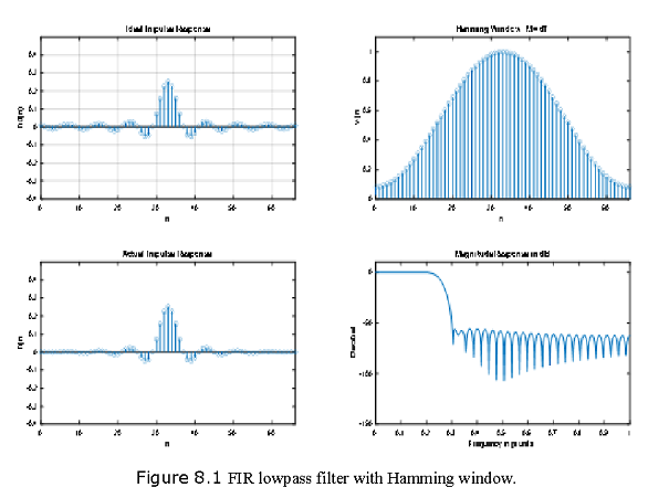
Example 7.8: Design a digital FIR lowpass filter with Hamming window. Following are the filter specifications:

\[ω_p=0.2π,R_p=0.25\] dB \[ω_s=0.3π,A_s=50\] dB

Hamming window:

\[\begin{equation} W(n)=\begin{cases} 0.54-0.46cos(\frac{2\pi n}{M-1}), 0\le n \le M-1, \\ 0, elsewhere \end{cases} \tag{8.6} \end{equation}\]

% Example 8.1 Disign a ditital FIR lowpass filter with the following specifications

wp = 0.2pi; ws = 0.3pi; tr_width = ws-wp;

M = ceil(6.6*pi/tr_width)+1

M = 67;

n = [0:1:M-1];

wc = (ws+wp)/2; % Ideal FPF cutoff frequency

hd = ideal_lp(wc,M);

w_ham = (hamming(M))’;

h = hd.*w_ham;

[db,mag,pha,grd,w] = freqz_m(h,[1]);

delta_w = 2*pi/1000;

Rp = -(min(db(1:1:wp/delta_w+1))); % Actual passband ripple

Rp = 0.0394

As = -round(max(db(ws/delta_w+1:1:501))) % Min stopband attenuation

As = 52;

% plotting commands follow

subplot(2,2,1); stem(n,hd); title(‘Ideal Impulse Response’);

grid

axis([0 M-1 -0.4 0.5]); xlabel(‘n’); ylabel(‘hd(n)’)

subplot(2,2,2); stem(n,w_ham); title(‘Hamming Window: M = 67’)

axis([0 M-1 0 1.1]); xlabel(‘n’); ylabel(‘w(n’)

subplot(2,2,3); stem(n,h); title(‘Actual Impulse Response’)

axis([0 M-1 -0.4 0.5]); xlabel(‘n’); ylabel(‘h(n’)

subplot(2,2,4); plot(w/pi,db); title(‘Magnitude Response in dB’)

axis([0 1 -150 10]); xlabel(‘Frequency in pi units’);

ylabel(‘Decibel’)