Lab-7 FIR Linear Phase Filter Design:
Name:Write down your name
Date: Date of report submission and date of lab performed
7.1 FIR filter specifications:
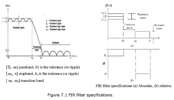
\(R_P\) is the passband ripple in dB \(A_S\) is the stopband attenuation in dB
\[\begin{equation} R_P=-20log_{10}\frac{1-\delta_1}{1+\delta_1} \space\space \gt 0 \tag{7.1} \end{equation}\]
\[\begin{equation} A_S=-20log_{10}\frac{\delta_2}{1+\delta_1} \space\space \gt 0 \tag{7.2} \end{equation}\]
Example 7.1: In a certain filter, RP = 0.25 dB, AS = 50 dB.
Determine \(δ_1\) and \(δ_2\).
Solution:
\[R_P=0.25=-20log_{10}\frac{1-\delta_1}{1+\delta_1}\]
\[δ_1=0.0144\] \[A_S=50=-20log_{10}\frac{\delta_2}{1+\delta_1}\] \[δ_2=0.0032\]
Example 7.2: Given the passband tolerance \(δ_1=0.01\) and the stopband tolerance \(δ_2=0.001\), determine the passband ripple \(R_P\) and the stopband attenuation \(A_S\).
Solution:
\[R_P=-20log_10\frac{(1-0.01)}{(1+0.01)}=0.1737\space dB\] \[A_S=-20log_{10}\frac{0.001}{1+0.01}=60\space dB\]
7.2 Properties of Linear-Phase FIR Filters:
In this section, we discuss shapes of impulse and frequency responses and locations of system function zeros of linear-phase FIR filters. Let h(n), \(0 \le n \le M-1\) , be the impulse response of length (or duration) M. Then the system function is
\[\begin{equation} H(z)=\sum_{k=0}^{M-1}h(n) z^{-n}= z^{-(M-1)} \sum_{k=0}^{M-1}h(n) z^{M-1-n} \tag{7.3} \end{equation}\]
which has (M-1) poles at the origin z = 0 (trivial poles) and (M-1) zeros located anywhere in the z-plane. The frequency response function is
\[\begin{equation} H(e^{jω} )=\sum_{k=0}^{M-1}h(n)e^{-jωn}\space\space -\pi \lt \omega \le π \tag{7.4} \end{equation}\]
Now we will discuss specific requirements on the forms of h(n) and \(H(e^{jω})\) as well as requirements on the specific locations of (M-1) zeros that the linear-phase constraint imposes.
7.3 Impulse Response h(n)
We impose a linear-phase constraint
\[\begin{equation} \angle H(e^{jω})=\angle H(ω) = -\alpha\omega,-\pi \lt \omega \le \pi \tag{7.5} \end{equation}\]
where \(\alpha\) is a constant phase delay. Then h(n) must be symmetric, that is
\[\begin{equation} h(n)=h(M-1-n); 0 ≤ n ≤(M-1)\space with\space \alpha =\frac{(M-1)}{2} \tag{7.6} \end{equation}\]
Hence h(n) is symmetric about \(\alpha\), which is the index of symmetry.
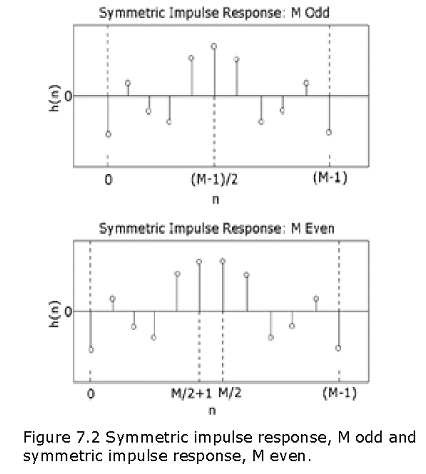
There are two possible types of symmetry:
M odd. In this case, \(\alpha=\frac{(M-1)}{2}\) is an integer. The impulse response is shown below:
M even. In this case, \(\alpha=\frac{(M-1)}{2}\) is not an integer. The impulse response is shown below:
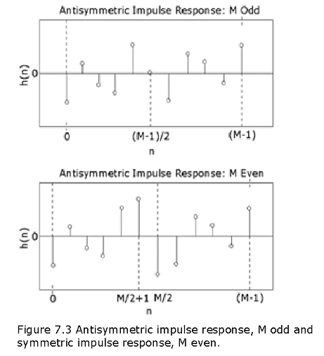
Impulse response h(n) is antisymmetric:
\[\begin{equation} h(n)=-h(M-1-n); 0 ≤ n ≤ M-1, \alpha = \frac{(M-1)}{2}, \beta = \pm \frac{\pi}{2} \tag{7.7} \end{equation}\]
There are two possible types of antisymmetry:
M odd. In this case, \(\alpha=\frac{(M-1)}{2}\) is an integer. The impulse response is shown below:
M even. In this case, \(\alpha=\frac{(M-1)}{2}\) is not an integer. The impulse response is shown below:
7.4 Frequency Response H(\(e^{jω}\))
When the cases of symmetry and antisymmetry are combined with odd and even M, we obtain four types of linear-phase FIR filters. Frequency response functions for each of these types have some peculiar expressions and shapes. To study these responses, we write H(\(e^{jω}\)) as
\[\begin{equation} H(e^{jω})=H_r(ω) e^{(-jω\frac{(M-1)}{2})};\beta = \pm \frac{\pi}{2},\alpha=\frac{(M-1)}{2} \tag{7.8} \end{equation}\]
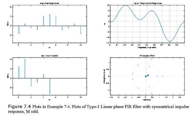
Type-1 Linear FIR filter: Symmetrical impulse response, M odd.
In this case \(\beta = 0,h(n)=h(M-1-n),0≤n≤M-1\),but \(\alpha = \frac{(M-1)}{2}\) is an integer.
The system function is given by
\[\begin{equation} H(e^{j\omega})=\left[\sum_{n=0}^{M-1}a(n)cos(\omega n)\right]e^{-j\omega (M-1)/2} \tag{7.9} \end{equation}\]
where sequence a(n) is obtained from h(n) as with \(α(0)=h\frac{(M-1)}{2}\) (the middle sample),
\[\begin{equation} α(n)=2h((M-1)/2-n), 1 ≤ n ≤ M-3/2 \tag{7.10} \end{equation}\]
Comparing (7.8) and (7.9), we get
\[\begin{equation} H_r(\omega)=\sum_{n=0}^{(M-1)/2}a(n)cos(\omega n) \tag{7.11} \end{equation}\]
Example 7.3
Let h(n)={\(\bar(-4)\),1,-1,-2,5,6,5,-2,-1,1,-4}. Determine the amplitude response H_r (ω) and the locations of the zeros of H(z).
Solution:
Since M = 11, which is odd, and since h(n) is symmetric about α=(M-1)/2=((11-1))/2=5, this is a Type-1 linear phase FIR filter.
From (7.7), we have
α(0)=h((M-1)/2)=h((11-1)/2)=h(5)=6 (the middle sample)
α(1)=2h((11-1)/2-1)=2h(4)=2(5)=10
α(2)=2h((11-1)/2-2)=2h(3)=2(-2)=-4
α(3)=2h((11-1)/2-3)=2h(2)=2(-1)=-2
α(4)=2h((11-1)/2-4)=2h(1)=2(1)=2
α(5)=2h((11-1)/2-5)=2h(0)=2(-4)=-8
Now from (7.8), we get
\[H_r(\omega)=\sum_{n=0}^{(M-1)/2}a(n)cos{(\omega n)}=\sum_{n=0}^5 a(n)cos(\omega n)\] \[H_r(\omega)=a(0)cos(0)+a(1)cos(\omega)+a(2)cos(2\omega)+a(3)cos(3\omega)+a(4)cos(4\omega)+a(5)cos(5\omega)\] \[H_r(\omega)=6+10cos(\omega)-4cos(2\omega)-2cos(3\omega)+2cos(4\omega)-8cos(5\omega)\] % Example 7.4 Type-1 Linear Filter
h = [-4,1,-1,-2,5,6,5,-2,-1,1,-4];
M = length(h); n = 0:M-1;
[Hr,w,a,L] = Hr_Type1(h);
amax = max(a) + 1; amin = min(a)-1;
subplot(2,2,1); stem(n,h); axis([-1 2*L+1 amin amax])
xlabel(‘n’); ylabel(‘h(n)’);title(‘impulse Response’)
subplot(2,2,3); stem(0:L,a); axis([-1 2*L+1 amin amax]) xlabel(‘n’); ylabel(‘a(n)’);title(‘a(n) coefficients’)
subplot(2,2,2); plot(w/pi,Hr); grid
xlabel(‘frequnecy in pi units’); ylabel(‘Hr’);title(‘Type-1 Amplitude Response’)
subplot(2,2,4); zplane(h,1)
xlabel(‘real axis’); ylabel(‘imaginary axis’);title(‘Pole-Zero Plot’)
function [Hr, w, a, L] = Hr_Type1(h);
M = length(h);
L = (M-1)/2;
a = [h(L+1) 2*h(L:-1:1)]; %1 x (L+1) row vector
n = [0:1:L]; %(L+1)x1 column vector
w = [0:1:500]’*pi/500;
Hr = cos(wn)a’;
Type-2 Linear FIR filter: Symmetrical impulse response, M even.
In this case \(\beta = 0,h(n)=h(M-1-n),0 ≤ n ≤ M-1\),but \(α=(M-1)/2\) is not an integer.
\(\beta = 0,h(n)=h(M-1-n),0 ≤ n ≤M-1,\space but\space \alpha=(M-1)/2\)
is not an integer.
\[\begin{equation} H(e^{j\omega})=\left[\sum_{n=1}^{M/2}b(n)cos\omega(n-1/2)e^{-j\omega(M-1)/2}\right] \tag{7.12} \end{equation}\]
with
\[\begin{equation} b(n)=2h(M/2-n),\space where \space n = 1,2,.....M/2. \tag{7.13} \end{equation}\]
Hence the magnitude is given by
\[\begin{equation} H_r(\omega)=\sum_{n=1}^{(M/2)}b(n)cos(\omega(n-1/2)) \tag{7.14} \end{equation}\]
Note: At ω=π,we get
\[\begin{equation} H_r(\pi)=\sum_{n=1}^{(M/2)}b(n)cos\pi(n-1/2)=0 \tag{7.15} \end{equation}\]
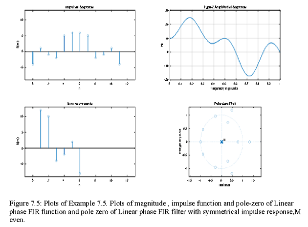
Example 7.5
Let h(n)={(-4)┬↑,1,-1,-2,5,6,6,5,-2,-1,1,-4} }. Determine the amplitude response H_r (ω) and the locations of the zeros of H(z).
Solution:
Since M = 12, which is even, and since h(n) is symmetric about α=(M-1)/2=((12-1))/2=5.5, this is a Type-2 linear phase FIR filter.
From (7.14), we have
b(n)=2h(M/2-n)
b(1)=2h(12/2-1)=2h(5)=2(6)=12
b(2)=2h(12/2-2)=2h(4)=2(5)=10
b(3)=2h(12/2-3)=2h(3)=2(-2)=-4
b(4)=2h(12/2-4)=2h(2)=2(-1)=-2
b(5)=2h(12/2-5)=2h(1)=2(1)=2
b(6)=2h(12/2-6)=2h(0)=2(-4)=-8
Now from (7.14), we get
\[H_r(\omega)=\sum_{n=1}^{(M/2)}b(n)cos\omega(n-1/2)=\sum_{n=1}^{(12/2)}b(n)cos(n-1/2)\] \[H_r(\omega)=b(1)cos\omega(1-1/2)+b(2)cos\omega(2-1/2)+b(3)cos\omega(3-1/2)+b(4)cos\omega(4-1/2)+b(5)cos\omega(5-1/2)+b(6)cos\omega(6-1/2)\]
\[H_r(\omega)=12cos(\omega/2)+10cos(3\omega/2)-4cos(5\omega/2)-2cos(7\omega/2)+2cos(9\omega/2)-8cos(11\omega/2)\]
% Example 7.5 Type-2 Linear Phase Filter
h = [-4,1,-1,-2,5,6,6,5,-2,-1,1,-4];
M = length(h); n = 0:M-1;
[Hr,w,b,L] = Hr_Type2(h);
bmax = max(b) + 1; bmin = min(b)-1;
subplot(2,2,1); stem(n,h); axis([-1 2*L+1 bmin bmax])
xlabel(‘n’); ylabel(‘h(n)’);title(‘impulse Response’)
subplot(2,2,3); stem(1:L,b); axis([-1 2*L+1 bmin bmax])
xlabel(‘n’); ylabel(‘b(n)’);title(‘b(n) coefficients’)
subplot(2,2,2); plot(w/pi,Hr); grid
xlabel(‘frequnecy in pi units’); ylabel(‘Hr’);title(‘Type-2 Amplitude Response’)
subplot(2,2,4); zplane(h,1)
xlabel(‘real axis’); ylabel(‘imaginary axis’);title(‘Pole-Zero Plot’)
function [Hr, w, b, L] = Hr_Type2(h);
M = length(h);
L = M/2;
b = 2*[h(L:-1:1)];
n = [1:1:L];n= n-0.5;
w = [0:1:500]’*pi/500;
Hr = cos(wn)b’;
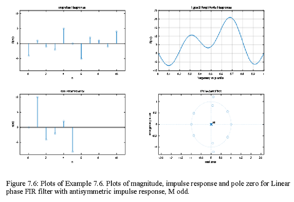
Type-3 Linear phase FIR filter with antisymmetric impulse response, M odd.
In this case β=π/2,α=((M-1))/2 is an integer, h(n)=-h(M-1-n), 0≤n≤M-1, and h (((M-1))/2)=0.
\[\begin{equation} H(e^{j\omega})=[\sum_{(n=1)}^{((M-1)/2)}c(n)sin\omega n]e^{(-j[\pi/2-\omega((M-1)/2)]} \tag{7.16} \end{equation}\]
\[\begin{equation} H(e^{j\omega})=[\sum_{(n=1)}^{((M-1)/2)}c(n)sin\omega n]e^{(-j[\pi/2-\omega((M-1)/2)])} \tag{7.17} \end{equation}\]
\[\begin{equation} c(n)=2h((M-1)/2-n),where \space n = 1,2,....,(M-1)/2. \tag{7.18} \end{equation}\]
The magnitude is given by \(((M-1))/2\).
\[\begin{equation} H_r(\omega)=\sum_{(n=1)}^{((M-1)/2)}c(n)sin\omega n. \tag{7.19} \end{equation}\]
% Example 7.6 Type-3 Linear Phase Filter
h = [-4,1,-1,-2,5,0,-5,2,1,-1,4];
M = length(h); n = 0:M-1;
[Hr,w,c,L] = Hr_Type3(h);
cmax = max(c) + 1; cmin = min(c)-1;
subplot(2,2,1); stem(n,h); axis([-1 2*L+1 cmin cmax])
xlabel(‘n’); ylabel(‘h(n)’);title(‘impulse Response’)
subplot(2,2,3); stem(0:L,c); axis([-1 2*L+1 cmin cmax])
xlabel(‘n’); ylabel(‘c(n)’);title(‘c(n) coefficients’)
subplot(2,2,2); plot(w/pi,Hr); grid
xlabel(‘frequnecy in pi units’);
ylabel(‘h(n)’);title(‘Type-3 Amplitude Response’)
subplot(2,2,4); zplane(h,1)
xlabel(‘real axis’); ylabel(‘imaginary axis’);title(‘Pole-Zero Plot’)
function [Hr, w, c, L] = Hr_Type3(h);
M = length(h);
L = (M-1)/2;
c = 2*[h(L+1:-1:1)];
n = [0:1:L];
w = [0:1:500]’*pi/500;
Hr = sin(wn)c’;
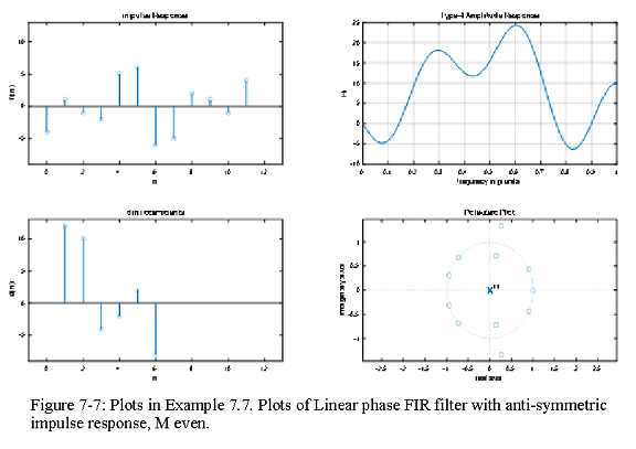
Type-4 Linear phase FIR filter with antisymmetric impulse response, M even.
\[\begin{equation} H(e^j\omega)=\left[\sum_{(n=1)}^{(M/2)}d(n)sin\omega (n-1/2)\right]e^{-j[\pi/2-\omega((M-1)/2)]} \tag{7.20} \end{equation}\]
where
\[\begin{equation} d(n)=2h(M/2-n),where \space n = 1,2,.....,M/2. \tag{7.21} \end{equation}\]
The magnitude is given by (M-1)/2.
\[\begin{equation} H_r(\omega)=\sum_{(n=1)}^(M/2)d(n)sin\omega (n-1/2). \tag{7.22} \end{equation}\]
In this case the magnitude is given by
\[\sum_{(n=1)}^{(M/2)}d(n)sin\omega(n-1/2)\]
% Example 7.7 Type-4 Linear Phase Filter
h = [-4,1,-1,-2,5,6,-6,-5,2,1,-1,4];
M = length(h); n = 0:M-1;
[Hr,w,d,L] = Hr_Type4(h);
dmax = max(d) + 1; dmin = min(d)-1;
subplot(2,2,1); stem(n,h); axis([-1 2*L+1 dmin dmax])
xlabel(‘n’); ylabel(‘h(n)’);title(‘impulse Response’)
subplot(2,2,3); stem(1:L,d); axis([-1 2*L+1 dmin dmax])
xlabel(‘n’); ylabel(‘d(n)’);title(‘d(n) coefficients’)
subplot(2,2,2); plot(w/pi,Hr); grid
xlabel(‘frequnecy in pi units’);
ylabel(‘Hr’);title(‘Type-4 Amplitude Response’)
subplot(2,2,4); zplane(h,1)
xlabel(‘real axis’); ylabel(‘imaginary axis’);title(‘Pole-Zero Plot’)
function [Hr, w, d, L] = Hr_Type4(h);
M = length(h);
L = M/2;
d = 2*[h(L:-1:1)];
n = [1:1:L]; n = n-0.5;
w = [0:1:500]’*pi/500;
Hr = sin(wn)d’;
Lab Assignments:
P.1 The absolute and relative (dB) specifications for a lowpass filter are related by (7.1) and (7.2). In this problem, we will develop a simple MATLAB function to convert one set of specifications into another.
- Write a MATLAB function to convert absolute specifications \(δ_1\) and \(δ_2\) into the relative specifications \(R_P\) and \(A_s\) in dB. The format of the function should be
- Verify your function using the specifications given in Example 7.2 (\(δ_1\)=0.01 and \(δ_2\)=0.001).
- Write a MATLAB function to convert relative specifications \(R_P\) and \(A_s\) in dB to absolute specifications \(δ_1\) and \(δ_2\). The format of the function should be
- Verify your function using the specifications given in Example 7.1 (\(R_P\) = 0.25 dB,\(A_s\) = 50 dB).
P.2 Write a MATLAB function to compute the amplitude response \(H_r(\omega)\) given a linear phase impulse response h(n). The format of the function should be
The function should first determine the type of the linear-phase FIR filter and then use the appropriate Hr_Type# function as discussed above. It should also check if the given h(n) is of a Linear-phase type. Verify the function on sequences given here.
\[h_1(n)=(0.9)^{|n-5|}cos[π(n-5)/12][u(n)-u(n-11)]\]
\[h_2(n)=(0.9)^{|n-4.5|}cos[π(n-4.5)/11][u(n)-u(n-10)]\]
\[h_3(n)=(0.9)^{|n-5|}sin[π(n-5)/12][u(n)-u(n-11)]\]
\[h_4(n)=(0.9)^{|n-4.5|}sin[π(n-4.5)/11][u(n)-u(n-10)]\]
\[h_5(n)= (0.9)^n cos[π(n-5)/12][u(n)-u(n-11)]\]