Lab-5 Inverse Z-transform

Name:Write down your name

Date: Date of report submission and date of lab performed

In Lab#4, we presented some important properties of the z-transform that are given below again.

PROPERTIES OF THE Z-TRANSFORM: The properties of the z-transform are generalizations of the properties of the discrete time Fourier transform. Linearity:

\[Z\{x_1 (n)+a_2 x_2 (n)\}=a_1 X_1 (z)+a_2 X_2 (z)\]

Sample shifting:

\[Z\{x(n-n_0)\}=z^{-n_0} X(z)\]

Frequency shifting:

\[Z\{a^n x(n)\}=X(z/a)\]

Folding:

\[Z\{x(-n)\}=X(1/z)\]

Complex conjugation:

\[X\{x^*(n)\}=X^* (z^*)\]

Differentiation in the z-domain:

\[Z\{nx(n)\}=-z \frac{dX(z)}{dz}\]

Convolution:

\[Z\{x_1 (n)*x_2 (n)\}=X_1 (z) X_2 (z)\]

Table 5.1 Some Common z-Transform Pairs.

Signal, x(n)	z-Transform, X(z)	ROC
\(\delta(n)\)	1	\(\forall z\)
u(n)	\(\frac{1}{(1-z^{-1})}\)	\(\|z\|\gt 1\)
\(a^nu(n)\)	\(\frac{1}{(1-az^{-1})}\)	\(\|z\|\gt \|a\|\)
\(na^nu(n)\)	\(\frac{az^{-1}}{(1-az^{-1})^2}\)	\(\|z\|\gt \|a\|\)
\(-a^nu(-n-1)\)	\(\frac{1}{(1-az^{-1})}\)	\(\|z\|\lt \|a\|\)
\(-na^nu(-n-1)\)	\(\frac{az^{-1}}{(1-az^{-1})^2}\)	\(\|z\|\lt \|a\|\)
\((cos\omega_0n)u(n)\)	\(\frac{1-z^{-1}cosω_0}{1-2z^{-1}cosω_0+z^{-2}}\)	\(\|z\|\gt 1\)
\((sin\omega_0n)u(n)\)	\(\frac{z^{-1}sinω_0}{1-2z^{-1}cosω_0+z^{-2}}\)	\(\|z\|\gt 1\)
\((a^ncos\omega_0n)u(n)\)	\(\frac{1-az^{-1}cosω_0}{1-2az^{-1}cosω_0+a^2z^{-2}}\)	\(\|z\|\gt a\)
\((a^nsin\omega_0n)u(n)\)	\(\frac{az^{-1}sinω_0}{1-2az^{-1}cosω_0+a^2z^{-2}}\)	\(\|z\|\gt a\)

Example 5.1

Using z-transform properties and the z-transform Table 3.3, determine the z-transform of

\[x(n)=(n-2)(0.5)^{(n-2)} cos[\pi/3 (n-2)]u(n-2)]\]

Solution: Applying the sample-shift property,

\[X(z)=Z[x(n)]= z^{-2} Z[n(0.5)^n cos(\pi n/3)u(n)]\]

with no change in the ROC. Applying the multiplication by a ramp property,

\[X(z)=z^{-2}\{-z\frac{d}{dz}[(0.5)^n cos(πn/3)u(n)]\}\]

with no change in ROC. Now the z-transform of \((0.5)^n cos(πn/3)u(n)\) from Table 5.1 is

\[Z[n(0.5)^n cos(πn/3)u(n)]= (1-(0.5)^{-1} cos(π/3))/(1-2(0.5)z^{-1} cos(π/3)+(0.5)^2 z^{-2}); |z|>0.5\]

\[=(1-(0.5)z^{-1} cos(π/3))/(1-2(0.5)z^{-1} cos(π/3)+(0.5)^2 z^{-2});|z|>0.5 \]
\[=1-(0.25)z^{-1}/(1-(0.5)z^{-1}+0.25z^{-2}); |z|>0.5\]

Hence, \[X(z)=-z^{-1} d/dz {1-(0.25)z^{-1}/(1-(0.5)z^{-1}+0.25z^{-2} )}\]

\[X(z)=-z^{-1} {(-0.25z^{-2}+0.5z^{-3}-0.0625z^{-4})/(1-z^{-1}+0.75z^{-2}-0.25z^{-3}+0.0625z^{-4})};|z|>0.5\]

\[={(0.25z^{-2}-0.5z^{-3}+0.0625z^{-4})/(1-z^{-1}+0.75z^{-2}-0.25z^{-3}+0.0625z^{-4})}; |z|>0.5\]

The above result can easily be verified using MATLAB by computing the first eight samples of the sequence x(n) corresponding to X(z),

b = [0,0,0,0.25,-0.5,0.0625];

a = [1,-1,0.75,-0.25,0.0625];

[delta, n] = impseq(0,0,7)

x = filter(b,a,delta) % check sequence

%check the result with original sequence

\[x=[(n-2)(1/2)^{n-2}cos(pi(n-2)/3)].\] stepseq(2,0,7)

Output: >> Example_5_1 delta =

1×8 logical array 1 0 0 0 0 0 0 0

n = 0 1 2 3 4 5 6 7

x = Columns 1 through 6

     0         0         0    0.2500   -0.2500   -0.3750

Columns 7 through 8

-0.1250 0.0781

x = Columns 1 through 6

     0         0         0    0.2500   -0.2500   -0.3750

Columns 7 through 8

-0.1250 0.0781

Given the z-transform X(z) of a signal and we need to determine the signal sequence. The procedure for transforming from the z-domain to the time domain is called the inverse z-transform. An inversion formula for obtaining x(n) from X (z) can be derived by using the Cauchy integral theorem. which is an important theorem in the theory of complex variables. To define the inverse z-transform we need to start with the z-transform of a discrete-time signal x(n) is defined as the power series

\[\begin{equation} X(z)=\sum_{k =-\infty}^{\infty}x(k)z^{-k} \tag{5.1} \end{equation}\]

Suppose that we multiply both sides of Eq.(5.1) by \(z^{-1}\) and inlegrate both sides over a closed contour within the ROC of X(z) which encloses the origin. Such a contour is illustrated in Fig. 5.1.

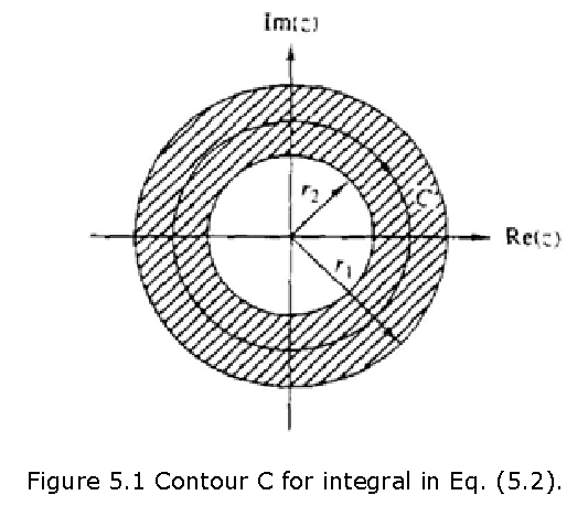
Thus we have

\[\begin{equation} \oint_c X(z) z^{n-1}dz =\oint_c\sum_{k=-\infty}^\infty x(k)z^{(n-1-k)} dz \tag{5.2} \end{equation}\]

\[\begin{equation} \oint_c X(z) z^{n-1}dz=\sum_{k=-\infty}^\infty x(k)\oint_c z^{n-1-k} dz \tag{5.3} \end{equation}\]

Now we can invoke the Cauchy integral theorem, which states that

\[\begin{equation} 1/2\pi j\oint_c z^{n-1-k}dz= \begin{cases} 1, k=n\\ 0, k\neq n \end{cases} \tag{5.4} \end{equation}\]

where C is any contour that encloses the origin. By applying (5.4), the righthand side of (5.3) reduces to 2πjx(n) and hence the desired inversion formula for the inverse z-transform of a complex function X(z) is given by:

\[\begin{equation} x(n)=Z^{-1} [X(z)]=1/2πj \oint_cX(z)z^{n-1} dz \tag{5.5} \end{equation}\]

where C is a counterclockwise contour encircling the origin and lying in the ROC.

Although the contour integral in (5.5) provides the desired inversion formula for determining the sequence x(n) from the z-transform, we shall not use (3.1.16) directly in our evaluation of inverse z-transforms. In our treatment we deal with signals and systems in the z-domain which have rational i-transforms (i.e., z-transforms that are a ratio of two polynomials). For such z-transforms we develop a simpler method for inversion that stems from (5.5) and employs a table lookup.

The complex variable z is called the complex frequency given by \(z= |z| e^{j\omega}\) where |z| is the attenuation and 𝜔 is the real frequency. The function |z| = 1 (or \(z = e^{j\omega}\) ) is a circle of unit radius in the z-plane and is called the unit circle. If the ROC contains the unit circle, then we can evaluate X(z) on the unit circle.

\[\begin{equation} X(z)|_{z=j\omega}=X(e^{j\omega}) =\sum_{n=-\infty}^{\infty}x(n)e^{-j\omega n} \tag{5.6} \end{equation}\]

z-Transform Using Partial Fraction Expansion Method:

The computation of the inverse z-transform using (5.6) involves an evaluation of complex contour integral that, in general is a complicated procedure. The most practical approach is to use the partial fraction expansion method.

When X(z) is a rational function of \(z^{-1}\), it can be expressed as a sum of simple factors using the partial fraction expansion. The individual sequences corresponding to these factors can then be written down using the z-transform table. The inverse z-transform procedure can be summarized using the following steps:

Consider the rational function

\[\begin{equation} X(z)=\frac{N(z)}{D(z)} = \frac{(b_0+b_1 z^{-1}+⋯+b_M z^{-M})}{(a_0+a_1 z^{-1}+⋯+a_N z^{-N} )} = \frac{\sum_{k=0}^M b_k z^{-k}}{\sum_{k=0}^N{a_k} z^{-k}}, R_{x-} < |z| < R_{x+} \tag{5.7} \end{equation}\]

Express (5.7) as

\[\begin{equation} X(z)=\frac{N(z)}{D(z)} =\underbrace{\frac{ (b_0+b_1 z^{-1}+⋯+b_M z^{-(N-1)})}{(a_0+a_1z^{-1}+⋯+a_Nz^{-N} )}}_\text{Proper rational part} + \underbrace{\sum_{k=0}^{M-N}C_k z^{-k})}_\text{Polynomial part if M ≥N} \tag{5.8} \end{equation}\]

where the first term on the right-hand side is the proper rational part and the second term is the polynomial (finite length) part. This can be obtained by performing polynomial division if M ≥N using deconv function.

Perform a partial expansion on the proper rational part of X(z) to obtain

\[\begin{equation} X(z)= \sum_{(k=1)}^N\frac{R_k}{(1-p_k z^{-1})}+\sum_{k=0}^{M-N}C_kz^{-k}┬(M ≥N) \tag{5.9} \end{equation}\]

where \(p_k\) is the kth pole of X(z) and \(R_k\) is the residue at \(p_k\). It is assumed that the poles are distinct, for which the residues are given by

\[\begin{equation} R_k=\frac{b_0+b_1 z^{-1}+....+b_Mz^{-(N-1)}}{a_0+a_1z^{-1}+....a_Nz^{-N}}(1-p_k z^{-1} )|_{z= p_k} \tag{5.10} \end{equation}\]

For repeated poles, the expansion (5.9) has a more general form. If a pole \(p_k\) has multiplicity r, then its expansion is given by

\[\begin{equation} \sum_{l=1}^r\frac{(R_{k,l} z^{-({l-1})}}{(1-p_k z^{-1} )^l} =\frac{R_{k,1}}{(1-p_k z^{-1})}+ \frac{R_{k,2}z^{-1}}{(1-p_k z^{-1})^2} +⋯+\frac{R_{k,r}z^{-(r-1)}}{(1-p_k z^{-1} )^r} \tag{5.11} \end{equation}\]

where the residues \(R_{k,l}\) are computed using a more general formula is available in reference.

Assuming distinct poles in (4.10), write x(n) as

\[\begin{equation} x(n)= \sum_{k=1}^N R_k Z^{-1} [1/(1-p_k z^{-1} )]+(\sum_{k=0}^{M-N}C_k \delta(n-k))┬(M ≥N) \tag{5.12} \end{equation}\]

Finally, use the relation from Table 4.1

\[\begin{equation} Z^{-1}\left[\frac{1}{1-p_kz^{-1}}\right]= \begin{cases} p_k^nu(n)\\ -p_k^nu(-n-1) \end{cases} \tag{5.13} \end{equation}\]

Example 5.2 Find the inverse z-transform of \(X(z)=\frac{z}{(3z^2-4z+1)}\).

Solution

We can write

\[X(z)=\frac{z}{3(z^2-4/3z+1/3)}=\frac{1/3z^{-1}}{1-4/3z^{-1}+1/3z^{-2}}=\frac{1/3z^{-1}}{(1-z^{-1})(1-1/3z^{-1})}\] \[X(z)=\frac{A_1}{(1-Z^{-1})}+\frac{A_2}{1-1/3z^{-1}}\] \[\frac{1}{3}z^{-1}=A_1(1-\frac{1}{3}z^{-1})+A_2(1-z^{-1})\] Hence, \(A_1=\frac{1}{2}\) and \(A_2=-\frac{1}{2}\). Therefore, \[X(z)=\frac{1}{2(1-z^{-1})}-\frac{1}{2(1-\frac{1}{3}z^{-1})}\].

One can observe that X(z) has two poles \(z_1=1\) and \(z_2=1/3\), and since ROC is not specified, there are three possible ROCs, as discussed below:

\(ROC_1:1< |z|< \infty\). Hence both poles are on the interior side of the \(ROC_1\), that is, \(|z_1 |\le ROC_{-}=1\) and \(|z_2 \le 1\). Hence from (5.13), \[x_1 (n)=\frac{1}{2} u(n)-\frac{1}{2}\left(\frac{1}{3}\right)^n u(n)\] which is a right-sided sequence.
\(ROC_2:0 < |z|< 1/3\). Here both poles are on the exterior side of the \(ROC_2\), that is, \(|z_1 |≥ ROC_{x+}=1/3\) and \(|z_2 |≥ 1/3\).Hence from (5.13),

\[x_2(n)=\frac{1}{2} \{-u(-n-1)\}-\frac{1}{2} \{-(\frac{1}{3})^n u(-n-1)\}\] \[x_2(n)=\frac{1}{2} \{(\frac{1}{3})^n u(-n-1)\}-\frac{1}{2} \{u(-n-1)\}\]

which is a left-sided sequence.

\(ROC_3:1/3< |z|< 1\). Here pole z_1 are on the exterior side of the \(ROC_3\), that is, \(|z_1 |≥ ROC_{x+}=1\) and pole \(z_2\) is on the interior side,that is |z_2 |≤( 1)/3. Hence from (5.13),

\[x_2 (n)=-\frac{1}{2} \{u(-n-1)\}-\frac{1}{2} \{(\frac{1}{3})^n u(n)\}\] which is a two-sided sequence.

MATLAB Implementation:

A MATLAB function residuez is used to compute the residue part and the direct (or polynomial) terms of a rational function in \(z^{-1}\). As given earlier in (5.9), a rational function in which the numerator and denominator polynomials are in ascending powers of \(z^{-1}\).

\[\begin{equation} X(z)= \sum_{(k=1)}^N\frac{R_k}{(1-p_k z^{-1})}+\sum_{k=0}^{M-N}C_kz^{-k}┬(M ≥N) \tag{5.9} \end{equation}\]

Therefore, calling [R,p,C] = residuez(b,a) will return the residues, poles and direct terms of X(z) in which two polynomials B(z) and A(z) are given in two vectors b and a, respectively. The returned column vector R contains the residues, column vector p contains the pole locations, and row vector C contains the direct terms.

Similarly, calling [b,a] = residuez(R,p,C) will convert the partial fraction back to polynomials with coefficients in row vectors b and a.

Example 5.3 To verify the residue calculations, let us consider the following rational function as given in Example 5.2.

\[X(z)=\frac{z}{(3z^2-4z+1)}\].

Solution: Rearranging X(z) so that it is a function in ascending powers of \(z^{-1}\).

\[\frac{(0+ z^{-1})}{(3-4z^{-1}+z^{-2} )}\].

Now, using the following MATLAB code from the Command line will give us the R, p and C to generate the partial function.

% Example 5.3 to calcutes residues, poles and direct terms.

b = [0,1]; a = [3,-4,1];

[R,p,C] = residuez(b,a)

% Output: % Example_5_3_residuez

% R =

% 0.5000

% -0.5000

% p =

% 1.0000

% 0.3333

% C =

% []

These outputs can be used to construct the rational function that we showed earlier in Example 5.2 mathematically.

\[X(z)= \frac{(\frac{1}{2})}{(1-z^{-1})} + \frac{(-\frac{1}{2})}{(1-\frac{1}{3} z^{-1})}\] [b,a] = residuez(R,p,C)

% Output

% b = % -0.0000 0.3333

% a = % 1.0000 -1.3333 0.3333

These outputs can be used to construct the original function given in Example 5.2, as follows:

\[X(z)= \frac{(0+1/3 z^{-1})}{(1-4/3 z^{-1}+1/3 z^{-2})}\].

System Function in the z-Domain:

\[\begin{equation} H(z) =Z[h(n)]=\sum_{n=-\infty}^\infty h(n) z^{-n}; R_{h-} < |z|< R_{h} \tag{5.14} \end{equation}\]

Using the convolution preperty as given in Lab-4 of the z-transform, the output transform Y(Z) is given by

Y(z) = H(z)X(Z) : \(ROC_(y)= ROC_h⋂ROC_x\)

Provided 〖ROC〗_x overlaps with \(ROC_h\). Therefore, a linear and time-invariant system can be represented in the z-domain by

\[X(z)\to H(z)\to Y(z)=H(z)X(z)\]

System Function From the Difference Equation Representation:

When LTI system are described by a difference equation

\[\begin{equation} y(n)=-\sum_{k=1}^N a_k y(n-k) +\sum_{k=0}^M b_k x(n-k) \tag{5.15} \end{equation}\]

\[\begin{equation} Y(z)\left[1+\sum_{k=1}^N a_k z^{-k}\right] =X(z)\left[\sum_{k=0}^M b_k z^{-k}\right] \tag{5.16} \end{equation}\]

\[\begin{equation} H(z)=\frac{Y(z)}{X(z)} =\frac{\sum_{k=0}^M b_k z^{-k}}{1+\sum_{k=1}^N a_k z^{-k}} \tag{5.17} \end{equation}\]

The system function Eqn. (5-17) can be expressed in the product form

\[\begin{equation} H(z)=\frac{Y(z)}{X(z)} =\frac{(\sum_{k=0}^M b_k z^{-k})}{(1+\sum_{k=1}^N a_k z^{-k})}= b_0\frac{(\prod_{k=1}^M(1-z_k z^{-1})}{(\prod_{k=1}^N (1-p_k z^{-1} )} \tag{5.18} \end{equation}\]

where \(z_k\)’s are the system zeros and \(p_k\)’s are the system poles. Thus H(z) (and hence an LTI) system can also be represented in the z-domain using a pole-zero plot.

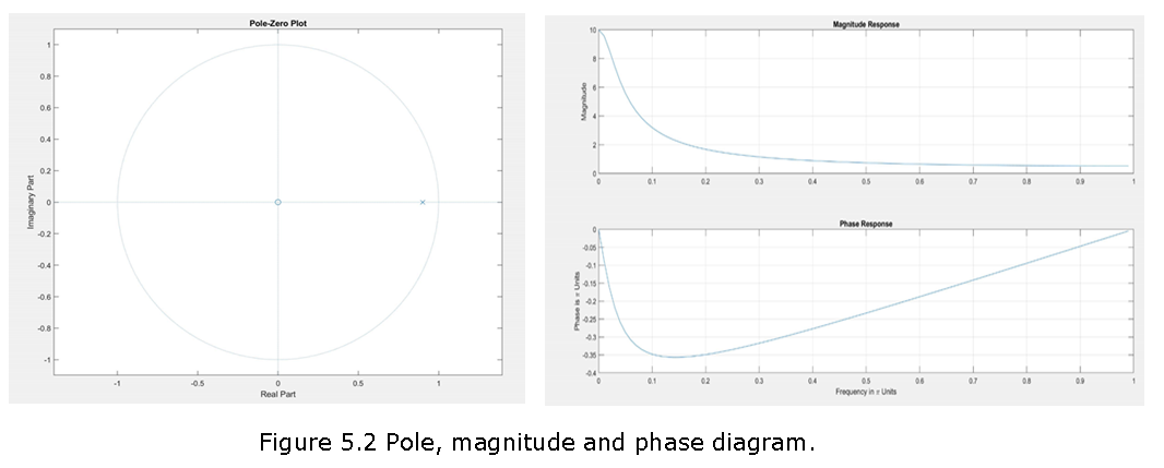
Example 4.11 Consider a causal system

y(n)=0.9y(n-1)+x(n)

Determine H(z) and sketch its pole-zero plot.
Plot |H(e^jω)| and \(\angle H(e^{jω})\).
Determine the impulse response h(n).

Solution: The difference equation can be put in the form y(n)-0.9y(n-1)=x(n)

\[H(z)=\frac{Y(z)}{X(z)}=\frac{1}{(1-0.9z^{-1})}; |z|\gt 0.9\]

Since the system is causal. There is one pole at 0.9 and one zero at the origin. We will use MATLAB to illustrate the use of the zplane function.

% Example 5.4 Causal system

% (a) b = [1,0]; a = [1, -0.9]; zplane(b,a)

% (b) [H,w] = freqz(b,a,100); magH = abs(H); phaH = angle(H);

subplot(2,1,1); plot(w/pi,magH); grid

title(‘Magnitude Response’); ylabel(‘Magnitude’);

subplot(2,1,2);plot(w/pi,phaH/pi); grid

xlabel(‘Frequency in Units’); ylabel(‘Phase is Units’);

title(‘Phase Response’)

Lab Assignment:

P.1 Determine the following inverse z-transform using the partial fraction expansion method

\(X_1 (z)=\frac{(1-z^{-1}-4z^{-2}+4z^{-3})}{(1-11/4 z^{-1}+13/8 z^{-2}-1/4 z^{-3})}\). The sequence is right shifted.
\(X_2(z)=\frac{(1+z^{-1}-4z^{-2}+4z^{-3})}{(1-11/4 z^{-1}+13/8 z^{-2}-1/4 z^{-3})}\). The sequence is absolutely summable.
\(X_3(z)=\frac{(z^3-3z^2+4z+1)}{(z^3-4z^2+z-0.16)}\). The sequence is right shifted.

P.2 A digital filter is described by the frequency response function \(H(e^jω )=\frac{(1+e^{-j4ω})}{(1-0.8145e^{-j4ω})}\).

Determine the difference equation representation.
Using the freqz function, plot the magnitude and phase of the frequency response of the filter. Note the magnitude and phase at ω=π/2 and at ω=π.
Generate 200 samples of the signal x(n)=sin(nπ/2)+5cos(πn), and process through the filter to obtain y(n). Compare the steady-state portion of y(n) to x(n). How are the amplitudes and phases of two sinusoids affected by the filter?

P.3 A digital filter is described by the frequency response function

\[H(e^{jω})=[1+2cos(ω)+3cos(2ω)]cos(ω/2) e^{-j5ω/2}\].

Determine the difference equation representation.
Using the freqz function, plot the magnitude and phase of the frequency response of the filter. Note the magnitude and phase at \(\omega=\pi/2\) and at \(\omega = \pi\).
Generate 200 samples of the signal \(x(n)=sin(n\pi/2)+5cos(\pi n)\), and process through the filter to obtain y(n). Compare the steady-state portion of y(n) to x(n). How are the amplitudes and phases of two sinusoids affected by the filter?