Lab-4 MATLAB implementation of Z-transform and LTI Systems
Name:Write down your name
Date: Date of report submission and date of lab performed
Review of z-transform:
The z-transform of a discrete-time signal x(n) is defined as the power series
\[X(z)=\sum_{n=-\infty}^\infty x(n)z^{-n}\]
where z is a complex variable. The short hand notation is
\[X(z)\equiv Z[x(n)]\]
\[x(n) \leftrightarrow^z X(z)\]
z-transform is an infinite power series, it exists only for those values of z for which this series converges, is called the region of convergence (ROC). The inverse z-transform of a complex function X(z) is given by:
\[x(n)=Z^{-1}[X(z)]=\frac{1}{2\pi j} \oint_c X(z)z^{n-1}dz\] where C is a counterclockwise contour encircling the origin and lying in the ROC.
The complex variable z is called the complex frequency given by \(z = |z|e^{j\omega}\) where |z| is the attenuation and 𝜔 is the real frequency. The function |z| = 1 (or z = \(e^{j\omega}\) ) is a circle of unit radius in the z-plane and is called the unit circle.
If the ROC contains the unit circle, then we can evaluate X(z) on the unit circle.
\[X(z)\vert_{z=j\omega}=X(e^{j\omega})=\sum_{n=-\infty}^\infty x(n)e^{-j\omega n}\]
PROPERTIES OF THE Z-TRANSFORM: The properties of the z-transform are generalizations of the properties of the discretetime Fourier transform. Linearity:
\[Z\{x_1 (n)+a_2 x_2 (n)\}=a_1 X_1 (z)+a_2 X_2 (z)\]
Sample shifting:
\[Z\{x(n-n_0)\}=z^{-n_0} X(z)\]
Frequency shifting:
\[Z\{a^n x(n)\}=X(z/a)\]
Folding:
\[Z\{x(-n)\}=X(1/z)\]
Complex conjugation:
\[X\{x^*(n)\}=X^* (z^*)\]
Differentiation in the z-domain:
\[Z\{nx(n)\}=-z \frac{dX(z)}{dz}\]
Convolution:
\[Z\{x_1 (n)*x_2 (n)\}=X_1 (z) X_2 (z)\]
The convolution property transforms the time-domain convolution operation into a multiplication between two functions. It is a significant property in many ways. First, if \(X_1(z)\) and \(X_2(z)\) are two polynomials, then their product can be implemented using the conv function in MATLAB.
Example-4-1:
Let \(X_1 (z)=2+3z^{-1}+4z^{-2}\) and \(X_2 (z)=3+4z^{-1}+5z^{-2}+6z^{-3}\).
Determine \(X_3 (z)=X_1(z)X_2(z)\).
Solution: From the given information, we find \(x_1 (n)=\{2,3,4\}\) and \(x_2 (n)=\{3,4,5,6\}\).
Using convolution property, we get the coefficients of the polynomial product using the following MATLAB code:
xl=[2,3,4]; x2=[3,4,5,6];
x3= conv(xl,x2)
x3 = 6 17 34 43 38 24
Hence \(X_3 (z)=6+17z^{-1}+34z^{-2}+43z^{-3}+38z^{-4}+24z^{-5}\)
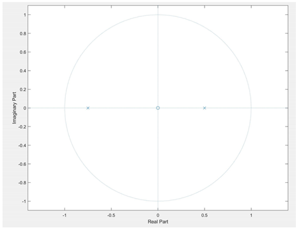
Example-4-2: Pole-zero plot calling zplane(z,p) function.
\[X(z) = \frac{z}{(z-0.5)(z+0.75)}\] ZPLANE Z-plane zero-pole plot. ZPLANE(Z,P) plots the zeros Z and poles P (in column vectors) with the unit circle for reference.
% MATLAB code
% Pole-zero plot of the above Example
z=[0]
p=[0.5; -0.75]
zplane(z,p)
Difference Equations:
An LTI discrete system can also be described by a linear constant coefficient difference equation of the form:
\[\sum_{k=0}^Na_ky(n-k)=\sum_{m=0}^Mb_mx(n-m)\space\space (1)\] \[a_0=1\] Another form of this equation is
\[y(n)=\sum_{k=1}^Na_ky(n-k)+\sum_{m=0}^Mb_mx(n-m)\space\space (2)\] A solution to this equation can be obtained in the form
\[y(n)=y_H(n)+y_P(n)\] The homogeneous part of the solution, y_H (n), is given by
\[y_H(n)=\sum_{k=1}^Nc_kz_k^n\]
where \(z_k\),k=1,…..,N are N roots (also called natural frequencies of the characteristic equation
\[\sum_{k=0}^Na_kz^{(N-k)}=0\] This characteristic equation is important in determining the stability of systems. If the roots \(z_k\) satisfy the condition \[|z_k|\lt 1, k = 1,2,...,N\] Then a causal system described by (2) is stable.
MATLAB implementation to solve difference equation is done by a function called filter. Given the input signal and the difference equation coefficients as given in the simplest form
y = filter(b,a,x) where \(b=[b_0,b_1,....,b_M]\) and \(a=[a_0,a_1,....,a_N]\);
are the coefficient arrays from the equation given in (1) and x is the input sequence array. The output y has the same length as input x. One must ensure that the coefficient \(a_0\) not be zero.
To compute and plot impulse response, MATLAB provides the function impz. When invoked by h = impz(b,a,n); it computes samples of the impulse response of the filter at the sample indices given in n with numerator coefficients in b and denominator coefficients in a.
Example-4-3:
Consider the following difference equation:
y(n)-y(n-1)+0.9y(n-2)=x(n); \(\forall n\)
Calculate and plot the impulse response h(n) at n = -20,……,100.
Calculate and plot the unit step response s(n) at n = -20,……,100.
Is the system specified by h(n) stable?
Solution:
From the given difference equation, with the coefficient arrays, we can solve the given problem using the following MATLAB code
% a. Plot of impulse response
% Solving difference equation
b = [1]; a = [1, -1, 0.9]; n = [-20:120];
% Coefficients
h = impz(b,a,n);
subplot(2,1,1); stem(n,h);
title(‘Impulse Response’); xlabel(‘n’);
ylabel(‘h(n)’);
% b. Plot of unit step response
x = stepseq(0,-20,120); s = filter(b,a,x);
subplot(2,1,2); stem(n,s)
title(‘Step Response’); xlabel(‘n’);
ylabel(‘s(n)’);
% Stability test
sum(abs(h))
% Alternate stability test
z = roots(a); magz = abs(z)
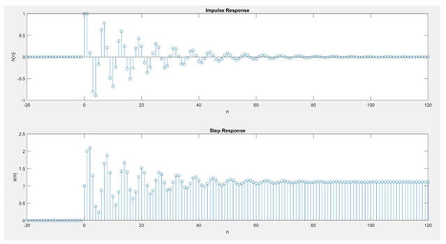
ans =
14.8785 Implies, the system is stable.
magz =
0.9487
0.9487
Since the magnitudes of both roots are less than 1, the system is stable.
Lab Assignment:
P.1. Determine the z-transform of the following sequences using MATLAB:
\(x(n)=(0.8)^nu(n-2)\). Verify the z-transform expression using MATLAB.
\(x(n)=[(0.5)^n+(-0.8)^n]u(n)\). Verify the z-transform expression using MATLAB.
\(x(n)=(n+1)3^nu(n)\). Verify the z-transform expression using MATLAB.
\(x(n)=2^ncos(0.4\pi n)u(-n)\)x(n)=2^n. Verify the z-transform expression using MATLAB.
Hints:
Example: Find z-transform of \(f=3n+n5^n\)f=n5^n+3n
syms n;
f = 3n + 5^nn
ztrans(f)
% ans =
syms z;
f=z/(z-3.0)+ (3*z)/(z-3.0)^2;
iztrans(f)
% ans = 23^n + 3^n(n - 1)
Output:
f = 3n + 5^nn
ans = (3z)/(z - 1)^2 + (5z)/(z - 5)^2 ans = 3n + 5^n + 5^n(n - 1)
P.2. Determine the results of the following polynomial operations using MATLAB.
\[X_1(z)= (1-2z^{-1}+3z^{-2}-4z^{-3} )(4+3z^{-1}-2z^{-2}+z^{-3})\]
\[X_2 (z)= (z^2-2z+3+2z^{-1}+z^{-2} )(z^3-z^{-3})\]
\[X_3(z)= (1+z^{-1}+z^{-2})^3\]
\[X_4(z)=X_1(z) X_2(z) +X_3(z)\]
Hints:
Example: Let \(X_1(z)=z+2+3z^{-1}\), and let \(X_2 (z)=2z^2+4z+3+5z^{-1}\).
Determine \(X_3 (z)= X_1 (z) X_2 (z)\).
Solution: We can find \(x_1(n)={1,2┬↑,3}\) and \(x_2 (n)={2,4,3┬↑,5}\).
Using the MATLAB code
% z-transform through convolution
x1 = [1,2,3]; n1 = [-1:1]; x2 = [2,4,3,5]; n2 = [-2:1];
[x3,n3] = conv_m(x1,n1,x2,n2)
Output: x3 = 2 8 17 23 19 15
n3 = -3 -2 -1 0 1 2
\[X_3 (z)=2z^3+8z^2+17z+23+19z^{-1}+15z^{-2}\]