Lab-6 Discrete Fourier Transform

Name:Write down your name

Date: Date of report submission and date of lab performed

The discrete-time Fourier transform and the z-transform are not numerically computable transforms. We try to find a numerically computable transform by sampling the discrete-time Fourier transform in the frequency domain (or the z-transform on the unit circle). We develop this transform by first analyzing periodic sequences. We know from Fourier analysis, that a periodic function (or sequence) can always be represented by a linear combination of harmonically related complex exponentials (which is a form of sampling). This gives us the discrete Fourier series (DFS) representation. Since the sampling is in the frequency domain, we study the effects of sampling in the time domain and the issue of reconstruction in the z-domain. We then extend the DFS to finite-duration sequences, which leads to a new transform, called the discrete Fourier transform (DFT). The numerical computation of the DFT for long sequences is very time-consuming. Alternative solution to this problem is to adapt several algorithms to effectively compute the DFT. These algorithms collectively called fast Fourier transform (or FFT) and two such algorithms we will study in detail.

The Discrete Fourier Series:

The condition for discrete signal \(\hat x(n)\) to be periodic is given by

\[\begin{equation} \hat x(n)=\hat x(n+kN) \tag{6.1} \end{equation}\]

where N is the fundamental period of the sequence. We know from Fourier analysis that the periodic function can be synthesized as a linear combination of complex exponentials whose frequencies are multiples or harmonics of the fundamental frequency (which in our case is 2π⁄N). From the frequency-domain periodicity of the discrete-time Fourier transform, we conclude that there are a finite number of harmonics; the frequencies are \({\frac{2π}{N}k, k=0,1,…..,N-1}\). Therefore, a periodic sequence x(n) can be expressed as

\[\begin{equation} \hat x(n)=\frac{1}{N}\sum_{k=0}^{N+1}\hat C(k)e^{i \frac{2\pi}{N}kn}, n = 0,\pm 1, \pm 2,..... \tag{6.2} \end{equation}\]

where \({\hat C(k),k=0,\pm 1,\pm 2,....}\) are called the discrete Fourier series coefficients, which are given by

\[\begin{equation} \hat C(k)=\sum_{k=0}^{N-1}\hat x(n) e^{-j \frac{2π}{N} kn},k=0,±1,….. \tag{6.3} \end{equation}\]

Note that \(\hat C(k)\) is itself a complex-valued periodic sequence with the fundamental period equal to N, that is,

\[\begin{equation} \hat C(k+N) = \hat C(k) \tag{6.4} \end{equation}\]

The pair of equations (6.1) and (6.2), together is called the discrete Fourier series representation of periodic sequences. Using \(W_N \triangleq e^{-j 2π/N}\) to denote the complex exponential term, we express (6.3) and (6.2) as

\[\begin{equation} \hat C(k)\triangleq DFS[\hat x(n)]=\sum_{n=0}^{N-1}\hat x(n) W_N^{nk} \tag{6.5} \end{equation}\]

Analysis or a DFS equation

\[\begin{equation} \hat x(n)\triangleq IDFS[\hat C(k)]=\frac{1}{N}\sum_{k=0}^{N-1} \hat x(n) W_N^{-nk} \tag{6.5} \end{equation}\]

Synthesis or an inverse DFS equation (6.5)

Example 6.1 Find the DFS representation of the periodic sequence \(\hat x(n)={……,0,1,2,3,\bar0,1,2,3,0,1,2,3,……}\).

Solution: The fundamental period of this sequence is N = 4.

Hence \(W_4=e^{-j 2π/4}=cos(2π/4)-jsin(2π/4)=-j\).

\[\hat C(k)=\sum_{n=0}^3\hat x(n) e^{-j \frac{2π}{4} nk}\]

\[\hat C(0)=\sum_{n=0}^3 \hat x(n) e^{-j \frac{2π}{4} n0}=\hat x(0)+\hat x(1)+\hat x(2)+\hat x(3)=0+1+2+3=6\]

\[\hat C(1)=\sum_{n=0}^3\hat x(n)e^{-j \frac{2\pi}{4}n}=\hat x(0)+\hat x(1)e^{-j 2π/4}+\hat x(2)e^{-j 2π/4 2}+\hat x(3)e^{-j 2π/4 3}=0-j-2+3j=-2+2j\]

\[\hat C(2)=\sum_{n=0}^3 \hat x(n)e^{-j 2π/4 n2}=\hat x(0)+\hat x(1) e^{-jπ}+\hat x(2) e^{-j2π}+\hat x(3) e^{-j3π}=0-1+2-3=-2\]

\[\hat C(3)=\sum_{n=0}^3\hat x(n)e^{-j 2π/4 n3}=\hat x(0)+\hat x(1) e^{-j 3π/2}+\hat x(2) e^{-j3π}+\hat x(3) e^{-j 9π/2}=0+j-2-3j=-2-2j\] MATLAB Implementation of Example 6.1

An efficient way to calculate DFS coefficients \(\hat C(k)\) in (5.5) is to use a matrix-vector multiplication for each of the relations in (5.5). Let bold letters x and C denote column vectors corresponding to the primary periods of sequences x(n) and C(k) respectively. Then (5.5) is given by

\[C=W_N x\] (6.6)

\[x =\frac{1}{N} W_N^*C\] (6.7)

Share where the matrix \(W_N\) is given by

\[W_N \triangleq \overbrace {\begin{bmatrix} 1 & 1 & 1 &...& 1 \\ 1 & W_N^1 & W_N^2 & ... & W_N^{N-1} \\ \vdots & ... & ... &\ddots & \vdots \\ 1 & W_N^{(N-1)} & W_N^{(N-2)} & ... & W_N^{(N-1)^2} \\ \end{bmatrix}}\]

The matrix \(W_N\) is a square matrix and is called a DFS matrix.

Matrix Method of Solving Example 6.1:

Using (6.6), we can get four linear equations to solve the discrete Fourier series coefficients as follows:

\[\begin{equation} \begin{bmatrix} \hat C(0) \\ \hat C(1) \\ \hat C(2) \\ \hat C(3) \\ \end{bmatrix} = \begin{bmatrix} W_4^{00} & W_4^{10} & W_4^{20} & W_4^{30} \\ W_4^{01} & W_4^{11} & W_4^{21} & W_4^{31} \\ W_4^{02} & W_4^{12} & W_4^{22} & W_4^{32} \\ W_4^{03} & W_4^{13} & W_4^{23} & W_4^{33} \\ \end{bmatrix} \begin{bmatrix} \hat x(0) \\ \hat x(1) \\ \hat x(2) \\ \hat x(3) \\ \end{bmatrix} \end{equation}\]

Solving \(W_N^{nk}=e^{-j \frac{2π}{N} kn}\) and making use of

\[\begin{equation} \begin{bmatrix} \hat x(0) \\ \hat x(1) \\ \hat x(2) \\ \hat x(3) \\ \end{bmatrix}= \begin{bmatrix} 0 \\ 1 \\ 2 \\ 3 \\ \end{bmatrix} \end{equation}\]

we can solve discrete Fourier series coefficients as follows:

\[\begin{equation} \begin{bmatrix} \hat C(0) \\ \hat C(1) \\ \hat C(2) \\ \hat C(3) \\ \end{bmatrix} = {\begin{bmatrix} 1 & 1 & 1 & 1 \\ 1 & -j & -1 & j \\ 1 & -1 & 1 & -1 \\ 1 & j & -1 & -j \\ \end{bmatrix}} \begin{bmatrix} 0 \\ 1 \\ 2 \\ 3 \\ \end{bmatrix} \end{equation}\]

\[\hat C(0)=6.0, \hat C(1)=-2+2j, \hat C(2)=-2, \hat C(3)=-2-2j\] Now, using (6.7) with the complex conjugate \(W_N^*\), we can get back the

\[\begin{equation} \begin{bmatrix} \hat x(0) \\ \hat x(1) \\ \hat x(2) \\ \hat x(3) \\ \end{bmatrix} = {\begin{bmatrix} 1 & 1 & 1 & 1 \\ 1 & -j & -1 & j \\ 1 & -1 & 1 & -1 \\ 1 & j & -1 & -j \\ \end{bmatrix}} \begin{bmatrix} 6 \\ -2+2j \\ -2 \\ -2-2j \\ \end{bmatrix} \end{equation}\]

\[\hat x(0)=0,\hat x(1)=1.0,\hat x(2)=2,\hat x(3)=3\]

The following MATLAB function dfs implements this matrix manipulation.

function [Ck] = dfs(xn,N)

% Computes discrete Fourier series coefficients

% ———————————————

% [Ck] = dfs(xn,N)

% Ck = DFS coefficients array over 0 <= k <= N-1

% xn = One period of periodic signal over 0 <= n <= N-1

% N = Fundamental period of xn

%

n = [0:1:N-1]; % Row vector for n

k = [0:1:N-1]; % Row vector for k

WN = exp(-i2pi/N); % Wn factor

nk = n’*k; % Creates an N by N matrix of nk values

WNnk = WN.^nk; % DFS matrix

Ck = xn*WNnk % Row vector for DFS coefficients

By calling dfs function, Example 5.1 is being computed as follows:

xn = [0,1,2,3]; N = 4; Ck = dfs(xn,N)

Ck = Columns 1 through 3

6.0000 + 0.0000i -2.0000 + 2.0000i -2.0000 - 0.0000i

Column 4

-2.0000 - 2.0000i

The following idfs function implements the synthesis equation.

function [xn] = idfs(Ck,N)

% Computes inverse discrete Fourier series coefficients

% ———————————————

% [xn] = idfs(Ck,N)

% xn = One period of periodic signal over 0 <= n <= N-1

% Ck = DFS coeff. array over 0 <= k <= N-1

% N = Fundamental period of Xk % n = [0:1:N-1]; % Row vector for n

k = [0:1:N-1]; % Row vector for k

WN = exp(-j2pi/N); % Wn factor

nk = n’*k; % Creates an N by N matrix of nk values

WNnk = WN.^(-nk); % IDFS matrix

Ck = xn*WNnk % Row vector for DFS coefficients

By calling idfs function, x(n) can be calculated in Example 5.1 as follows:

Ck = [6,-2+2j,-2,-2-2j]; N = 4; xn = idfs(Ck,N)

Output:

xn = Columns 1 through 3 0.0000 + 0.0000i 1.0000 + 0.0000i 2.0000 - 0.0000i

Column 4 3.0000 - 0.0000i

Example 6.2

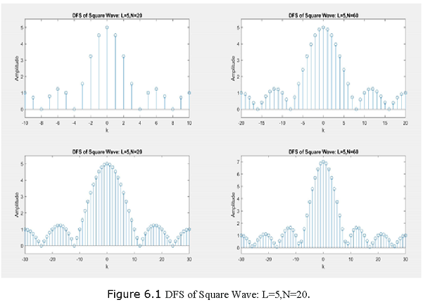
A periodic “square wave” sequence is given by \[ \begin{equation} \hat x(n)= \begin{cases} 1 \space\space\space mN\le n \le mN+L-1\\ 0 \space\space\space mN+L \le n \le (m+1)N-1 \end{cases} m = \pm 0, \pm 1, \pm 2..... \end{equation}\]

where N is the fundamental period and L/N is the duty cycle. (a) Determine an expression for |C ̂(k)| in terms of L and N.

2. Plot the magnitude |C ̂(k)| for L = 5, N = 20; L = 5, N = 40; L = 5, N = 60; L = 7, N = 60.

3. Comment on the results.

Solution: A plot of the sequence for L = 5 and N = 20 is shown in Figure 6.1.

1. By applying the analysis equation (6.3),

\[\hat C(k)=\sum_{k=0}^{N-1}\hat x(n) e^{-j {2π/N} kn} =\sum_{k=0}^{L-1}e^{-j {2π/N} kn} =\sum_{k=0}^{L-1}(e^{-j 2π/N k} )^n\] \[\begin{equation} \hat C(k)= \begin{cases} L \space\space\space k=0,\pm N,\pm 2N....... \frac{1-e^{-j2\pi Lk/N}}{1-e^{-j2\pi k/N}} \space\space\space, otherwise \end{cases} \end{equation}\]

The last step follows from the sum of the geometric terms formula (2.7) in Chapter 2. The last expression can be simplified to

\[\frac{(1-e^{-j2πLk/N})}{(1-e^{-j2πk/N})}=\frac{e^{-j2πLk/N}}{e^{-j2πk/N}} \frac{(e^{j2πLk/N}-e^{-j2πLk/N})}{(e^{j2πk/N}-e^{-j2πk/N} )}=e^{-j2π(L-1)k/N} \frac{sin(πkL/N)}{sin(πk/N)}\]

or the magnitude of \(\hat C(k)\) is given by

\[\begin{equation} \hat C(k)= \begin{cases} L \space\space\space k=0,\pm N,\pm 2N.......\\ \bigg|\frac{sin\frac{\pi kL}{N}}{sin\frac{\pi k}{N}}\bigg| \space\space\space, otherwise \end{cases} \end{equation}\]

2. The MATLAB script for L =5 and N = 20:

% Example 6.2

L = 5; N = 20; k = [-N/2:N/2]; % Square wave parameters xn = [ones(1,L),zeros(1,N-L)];

Ck = dfs(xn,N); %DFS

magCk = abs([Ck(N/2+1:N) Ck(1:N/2+1)]); %DFS magnitude

subplot(2,2,1); stem(k,magCk); axis([-N/2,N/2,-0.5,5.5])

xlabel(‘k’); ylabel(‘Amplitude’)

title(‘DFS of Square Wave: L=5,N=20’)

Lab Assignments:

Compute the DFS coefficients of the following periodic sequences using the DFS definition, and then verify the answers using MATLAB code.

i.\(\hat x_1(n)=\{4,1,-1,1\}\),N=4

Sample solution:

\[\begin{equation} \begin{bmatrix} \hat C(0) \\ \hat C(1) \\ \hat C(2) \\ \hat C(3) \\ \end{bmatrix} = \begin{bmatrix} W_4^{00} & W_4^{10} & W_4^{20} & W_4^{30} \\ W_4^{01} & W_4^{11} & W_4^{21} & W_4^{31} \\ W_4^{02} & W_4^{12} & W_4^{22} & W_4^{32} \\ W_4^{03} & W_4^{13} & W_4^{23} & W_4^{33} \\ \end{bmatrix} \begin{bmatrix} \hat x(0) \\ \hat x(1) \\ \hat x(2) \\ \hat x(3) \\ \end{bmatrix} \end{equation}\]

Solving \(W_N^{nk}=e^{-j \frac{2π}{N} kn}\) and making use of

\[\begin{equation} \begin{bmatrix} \hat x(0) \\ \hat x(1) \\ \hat x(2) \\ \hat x(3) \\ \end{bmatrix}= \begin{bmatrix} 4 \\ 1 \\ -1 \\ 1 \\ \end{bmatrix} \end{equation}\]

we can solve discrete Fourier series coefficients as follows:

\[\begin{equation} \begin{bmatrix} \hat C(0) \\ \hat C(1) \\ \hat C(2) \\ \hat C(3) \\ \end{bmatrix} = {\begin{bmatrix} 1 & 1 & 1 & 1 \\ 1 & -j & -1 & j \\ 1 & -1 & 1 & -1 \\ 1 & j & -1 & -j \\ \end{bmatrix}} \begin{bmatrix} 4 \\ 1 \\ -1 \\ 1 \\ \end{bmatrix} ={\begin{bmatrix} 4 + 1 - 1 + 1 \\ 4 -j + 1 + j \\ 4 -1 - 1 -1 \\ 4 + j + 1 -j \\ \end{bmatrix}} = \begin{bmatrix} 5 \\ 5 \\ 1 \\ 5 \\ \end{bmatrix} \end{equation}\]

\[\hat C(0)=5.0, \hat C(1)=5, \hat C(2)=1, \hat C(3)=5\]

ii.\(\hat x_2(n)=\{2,0,0,0,-1,0,0,0\}\),N=8

iii.\(\hat x_3(n)=\{1,0,-1,-1,0\}\),N=5

iv.\(\hat x_4(n)=\{0,0,2j,0,2j,0\}\),N=6

v.\(\hat x_5(n)=\{3,2,1\}\),N=3

% Part 1

% DSP Lab 6 Part 1

% Verify using MATLAB —————–

fprintf(“i————”)

xn=[4,1,-1,1]; N=4; Ck=dfs(xn,N)

fprintf(“ii————”)

xn=[2,0,0,0,-1,0,0,0]; N=8; Ck=dfs(xn,N)

fprintf(“iii————”)

xn=[1,0,-1,-1,0]; N=5; Ck=dfs(xn,N)

fprintf(“iv————”)

xn=[0,0,2i,0,2i,0]; N=6; Ck=dfs(xn,N)

fprintf(“v————”)

xn=[3,2,1]; N=3; Ck=dfs(xn,N)

% Part 2

% DSP Lab 6 Part 2

fprintf(“i.——”)

Ck=[4,3i,-3i]; N=3; xn=idfs(Ck,N)

fprintf(“ii.——”)

Ck=[i, 2i, 3i, 4*i]; N=4; xn=idfs(Ck,N)

fprintf(“iii.——”)

Ck=[1,2+3i,4,2-3i]; N=4; xn=idfs(Ck,N)

fprintf(“iv.——”)

Ck=[0,0,2,0,0]; N=5; xn=idfs(Ck,N)

fprintf(“v.——”)

Ck=[3,0,0,0,-3,0,0,0]; N=8; xn=idfs(Ck,N)

Output:

Lab_6

Part-I: i————

Ck = {5.0000 + 0.0000i , 5.0000 + 0.0000i, 1.0000 - 0.0000i, 5.0000 + 0.0000i}

ii————

Ck = {1.0000 + 0.0000i, 3.0000 + 0.0000i, 1.0000 - 0.0000i, 3.0000 + 0.0000i, 1.0000 - 0.0000i, 3.0000 + 0.0000i, 1.0000 - 0.0000i , 3.0000 + 0.0000i}

iii————

Ck = { -1.0000 + 0.0000i, 2.6180 + 0.0000i, 0.3820 - 0.0000i, 0.3820 + 0.0000i, 2.6180 + 0.0000i}

iv————

Ck = {0.0000 + 4.0000i, 0.0000 - 2.0000i, 0.0000 - 2.0000i, -0.0000 + 4.0000i, 0.0000 - 2.0000i, 0.0000 - 2.0000i}

v————

Ck = {6.0000 + 0.0000i, 1.5000 - 0.8660i, 1.5000 + 0.8660i}

Part-II:

i.—— xn = {1.3333 + 0.0000i, -0.3987 + 0.0000i, 3.0654 - 0.0000i}

ii.—— xn = {0.0000 + 2.5000i, 0.5000 - 0.5000i, -0.0000 - 0.5000i, -0.5000 - 0.5000i}

iii.—— xn = {2.2500 + 0.0000i, -2.2500 + 0.0000i, 0.2500 + 0.0000i, 0.7500 - 0.0000i}

iv.—— xn = {0.4000 + 0.0000i, -0.3236 + 0.2351i, 0.1236 - 0.3804i, 0.1236 + 0.3804i -0.3236 - 0.2351i}

v.—— xn = {0.0000 + 0.0000i, 0.7500 - 0.0000i, 0.0000 + 0.0000i, 0.7500 - 0.0000i, 0.0000 + 0.0000i, 0.7500 - 0.0000i, 0.0000 + 0.0000i, 0.7500 - 0.0000i}