Lab-9 IIR Filter Design
Name: Write down your name
Date: Date of report submission and date of lab performed
A linear time-invariant (LTI) system is characterized by its impulse response h(n). Also, linear time-invariant systems can be divided into two types, those that have a finite-duration impulse response we call them finite impulse response (FIR) and those that have an infinite-duration impulse response we call them infinite impulse respone (IIR). Thus an FIR system has an impulse response that is zero outside of some finite time interval.
The general form of the system function contains both poles and zeros and hence the corresponding system is called a pole-zero system, with N poles and M zeros. The pole-zero system sometime called IIR system due to prence of poles. A general system function can be divided into two parts one containg only poles we call them FIR and the other containing only poles we call them IIR. Due to the presence of poles, a pole-zero system is an IIR system.
General linear constant-coefficient difference equation as is given by:
\[\begin{equation} y(n)=-\sum_{k=1}^N a_k y(n-k)+\sum_{k=0}^M b_k x(n-k) \tag{9.1} \end{equation}\]
equivalently,
\[\begin{equation} y(n)=-\sum_{k=0}^N a_k y(n-k)+\sum_{k=0}^M b_k x(n-k), a_0 = 1 \tag{9.2} \end{equation}\]
By taking z-transform of Eqn. (9.2), one can get the system function H(z) as follows:
\[\begin{equation} H(z)=\frac{Y(z)}{X(Z)}=\frac{\sum_{k=0}^M b_k z^{-k}}{1+\sum_{k=1}^N a_k z^{-k}} \tag{9.3} \end{equation}\]
If \(b_k=0\) for \(1\le k \le M\)
\[\begin{equation} H(z)=\frac{Y(z)}{X(Z)}=\frac{b_0}{1+\sum_{k=1}^N a_k z^{-k}}=\frac{b_0z^N}{1+\sum_{k=1}^N a_k z^{N-k}}, a_0 \equiv 1 \tag{9.4} \end{equation}\]
Presence of poles, makes impulse response infinite in dimension and hence it is IIR system.
If \(a_k=0\) for \(1 \le k \le N\)
\[\begin{equation} H(z)=\frac{Y(z)}{X(Z)}=\sum_{k=0}^M b_k z^{-k} \tag{9.5} \end{equation}\]
Presence of zeros, makes impulse response finite in dimension and hence it is FIR system.
9.1 Some Special Types of Filters
In this section, we consider the design of some special types of digital filters with their characteristics.
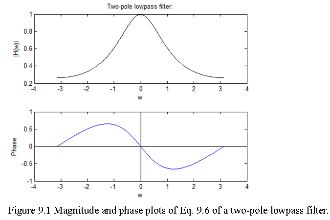
Example 9.1: A two-pole lowpass filter has the system function \(H(z)=\frac{b_0}{(1-pz^{-1} )^2}\). Determine the values of \(b_0\) and p such that the frequency response \(H(\omega)\) satisfies the conditions H(0)=1 and \(|H(\pi/4)|^2\)=1/2.
Solution:
\[H(\omega)=\frac{b_0}{(1-pe^{-jω})^2}\]. \[H(0)=\frac{b_0}{(1-p)^2} =1 \space or \space b_0=(1-p)^2\] At \(\omega = \frac{\pi}{4}\)
\[\frac{1}{\sqrt 2}=H(\frac{\pi}{4})=\frac{(1-p)^2}{[(1-p cos(\pi⁄4)+jpsin(\pi/4)]^2}\] \[\frac{1}{\sqrt 2}\frac{1}{\sqrt 2}=H(\frac{\pi}{4})H^*(\frac{\pi}{4})=\frac{(1-p)^4}{[1-pcos(\pi/4)+jpsin(\pi/4)]^2[(1-pcos(\pi/4)-jpsin(\pi/4)]^2]^2}\] \[\frac{1}{2}=\frac{(1-p)^4}{[(1-p/\sqrt{2})^2+(p/\sqrt{2})^2]^2}\] \[p^2[\sqrt{2}-1]+p[\sqrt{2}-2\sqrt{2}]+(\sqrt{2}-1)=0\] p=0.32 or 3.09
\[\begin{equation} H(z) = \frac{(1-p)^2}{(1-pz^{-1})^2}=\frac{(1-0.32)^2}{(1-0.32z^{-1})^2}=\frac{0.46}{(1-0.32z^{-1})^2} \tag{9.6} \end{equation}\]
MATLAB Implementation:
% % Example-9.1
w = [-pi:0.01:pi];
num = 0.46;
den = (1-0.32exp(-jw)).(1-0.32exp(-j*w));
Hw = num./den;
subplot(2,1,1)
plot(w,abs(Hw),‘black’);
xlabel(‘w’);
ylabel(‘|H(w)|’);
title(‘Two-pole lowpass filter:’);
subplot(2,1,2);
plot(w,angle(Hw));
line([-4 4],[0 0],‘Color’,‘k’,‘LineWidth’,1) % Horizontal line
line([0 0],[-1 1],‘Color’,‘k’,‘LineWidth’,1) % Horizontal line
xlabel(‘w’);
ylabel(‘Phase’);
Example 9.2
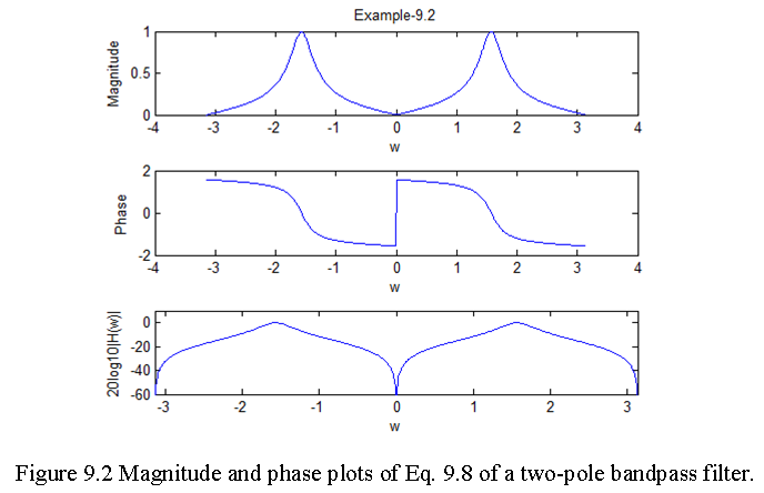
Design a two-pole bandpass filter that has the center of its passband at \(\omega = \pi/2\), zero in its frequency response characteristic at \(\omega=0\) and \(\omega=\pi\), and a magnitude of \(1/\sqrt{2}\) at \(\omega = 4\pi/9\).
Solution: The system function of a two-pole bandpass filter with poles \(p_{1,2}=re^{±j \pi⁄2}\) and zeros at z = 1 and z = -1 can be found as follows:
\[\begin{equation} H(z) = b_0\frac{\prod_{k=1}^M(1-z_kz^{-1})}{\prod_{k=1}^N(1-p_kz^{-1}}=G\frac{(z-1)(z+1)}{(z-jr)(z+jr)}=G\frac{z^2-1}{z^2+r^2} \tag{9.7} \end{equation}\]
The gain factor is determined by evaluating the frequency response \(H(\omega)\) of the filter at \(\omega = \pi/2\). Thus, we have
\[H(\omega)=G\frac{e^{j2\omega}-1}{e^{j2\omega}-r^2}\] \[H(\pi/2)=1=G\frac{e^{j2(\pi/2)}-1}{e^{j2(\pi/2)}-r^2}=G\frac{2}{1-r^2}\] \[G = \frac{(1-r^2)}{2}\] \[H(\omega)=\frac{1-r^2}{2}\frac{(e^{j2ω}-1)}{(e^{j2ω}-r^2)}\] \[H(\omega)H^*(\omega)=\frac{(1-r^2)^2}{4}\frac{(e^{j2ω}-1)}{(e^{j2ω}-r^2)}\frac{(e^{-j2ω}-1)}{(e^{-j2ω}-r^2)}\] \[|H(\omega)|^2=\frac{(1-r^2)^2}{4}\frac{2-2cos(2\omega)}{1+r^4+2r^2cos(2\omega)}\] The value of r is determined by evaluating \(H(\omega)\) of the filter at \(\omega = 4\pi/9\). Thus we have
\[|H(4\pi/9)|^2=\frac{(1-r^2)^2}{4}\frac{2-2cos(8\pi/9)}{1+r^4+2r^2cos(8\pi/9)}=\frac{1}{2}\] or, equivalently, \(1.94(1-r^2 )^2=1-1.88r^2+r^4\) From the given conditions \(r^2=0.7\) and gain, G = 0.15 and the system function
\[H(z)= 0.15\frac{(1-z^{-2})}{(1+0.7z^{-2})}\] and the corresponding system function as a function of \(\omega\) becomes
\[\begin{equation} H(\omega)= 0.15\frac{(1-e^{-j2\omega})}{(1+0.7e^{-j2\omega})} \tag{9.8} \end{equation}\]
MATLAB Implementation:
% Example 9.2
w = [-pi:0.01:pi];
num = [1.0 0 -1.0];
den = [1 0 0.7];
h = freqz(num,den,w);
subplot(3,1,1)
plot(w,abs(0.15*h));
xlabel(‘w’);
ylabel(‘Magnitude’);
title(‘Example-9.2’);
subplot(3,1,2);
plot(w,angle(h));
xlabel(‘w’);
ylabel(‘Phase’);
subplot(3,1,3);
plot(w,20log10(abs(0.15h)));
xlabel(‘w’);
ylabel(‘20log10|H(w)|’);
axis([-pi pi -60 10])
The magnitude and phase plots of Eq. (9.8) are:
9.1.1 Digital Resonators
A digital resonator is a two-pole bandpass filter. The system function of a digital resonator is given by
\[H(z)=\frac{b_0}{\prod(1-p_k z^{-1})} = \frac{b_0}{(1-p_1 z^{-1})(1-p_2 z^{-1})}\] considering the poles, \(p_1\) and \(p_2\)
\[p_{1,2} =re^{±jω_0}\] the system function can be expressed as
\[H(z)=\frac{b_0}{(1-re^{jω_0} z^{-1})(1-re^{-jω_0} z^{-1})}\]
\[H(z)=\frac{b_0}{(1-2re^{jω_0} z^{-1}+r^2 z^{-2})}\]
Since, \(|H(\omega)|\) peaks at the \(\omega = \omega_0\), we find gain, \(b_0\), so that \(|H(\omega_0)|\) = 1.
\[H(ω_0 )=\frac{b_0}{(1-re^{jω_0} e^{-jω_0} )(1-re^{-jω_0 } e^{-jω_0 } )}\] \[=\frac{b_0}{(1-r)(1-r e^{-j2 \omega_0 } ) }\]
\[|H(\omega_0)|=1=\frac{b_0}{(1-r)\sqrt{1+r^2-2rcos2\omega_0}}\] \[b_0 = (1-r)\sqrt{1+r^2-2rcos2\omega_0}\] \[|H(\omega_0)=1=\frac{b_0}{\sqrt{(1+r^2-2rcos (\omega_0-\omega )}\sqrt{(1+r^2-2rcos(\omega_0+\omega)})}\] \[|H(\omega)|=\frac{b_0}{U_1(\omega) U_2(\omega)}\]
\[U_1(\omega)U_2(\omega)\] reaches its minimum at the frequency
\[\begin{equation} \omega_r=cos^{-1}\frac{(1+r^2)}{2rcos(\omega_0)} \tag{9.9} \end{equation}\]
which defines the resonant frequency of the filter. A quantitative measure of the sharpness of the resonance is provided by the 3-dB bandwidth Δωof the filter. For values of r close to unity
\[\begin{equation} Δω≈2(1-r) \tag{9.10} \end{equation}\]
9.1.2 Notch Filters
A notch filter is a filter that contains one or more deep notches or ideally, perfect nulls in its frequency response characteristic:
In the instrumentation and recording systems require that the power line frequency of 60 Hz and its harmonics be eliminated.
To create a null, a pair of complex conjugate zeros on the unit circle at an angle \(\omega_0\).
\[z_{1,2}=e^{±j\omega_0}\] \[\begin{equation} H(z)=b_0(1-e^{j\omega_0}z^{-1})(1-e^{-j\omega_0}z^{-1}) \tag{9.11} \end{equation}\]
Suppose that we place a pair of complex conjugate poles at
\[p_{1,2}=re^{±j\omega_0}\] \[\begin{equation} H(z)=\frac{b_0(1-2cos\omega_0 z^{-1}+z^{-2})}{1-2rcos\omega_0 z^{-1}+r^2 z^{-2}} \tag{9.12} \end{equation}\]
9.1.3 Comb Filters:
A comb filter can be viewed as a notch filter in which the nulls occur periodically across the frequency band. To illustrate a simple comb filter, consider a moving average (FIR) filter
\[\begin{equation} y(n) = \frac{1}{(M+1}\sum_{k=0}^M x(n-k) \tag{9.13} \end{equation}\]
\[\begin{equation} H(z) = \frac{1}{(M+1)}\sum_{k=0}^M z^{-k}=\frac{1[1-z^{-(M+1)}]}{1-z^{-1}} \tag{9.14} \end{equation}\]
\[\begin{equation} H(\omega) = \frac{e^{-j\omega M/2} sin\omega \left(\frac{M+1}{2}\right)}{(M+1)sin(\omega/2)} \tag{9.15} \end{equation}\]
From Eq. (9.15) we observe that the filter has zeros on the unit circle at
\[z = \frac{e^{j2\pi k}}{(M+1)}\], k = 1,2,3,…..M
Note that the pole at z = 1 is actually cancelled by the zero at z = 1, so that in effect the FIR filter does not contain poles outside z = 0.
A plot of Eq. (9.15) for M = 10.