Lab-10 Sampling Rate Conversion
Name: Write down your name
Date: Date of report submission and date of lab performed
10.1 Introduction
In dealing with signal processing sometimes it requires to increase or decrease the sampling rate of a signal. The process of applying multiple sampling rates in the digital signal processing is called multirate digital signal processing.
In this lab students are going to be exposed with sampling down rate conversion called decimation and up rate conversion is called interpolation by integer factors. Sampling rate conversion has many applications in digital filters, subband coding of speech signals, transmultiplexing and oversampling A/D and D/A converters.
10.2 Decimation by a Factor D
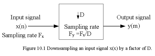
Decimation or downsampling of the high-rate signal x(n) into a low-rate signal y(m) with their corresponding time and frequency-domain relationship for error free decimation. In the decimation the downsampled signal y(m) is obtained from D samples of x(x) and throwing away the other (D-1) samples out of every D samples and can be expressed mathematically as follows:
\[\begin{equation} y(m) = \left. x(n)\right|_{n=md} = x(mD); n,m,D \in {integers} \tag{10.1} \end{equation}\]
The block diagram of Eq. (10.1) can be shown in Figure 10.1.
Example 10.1 Downsample the signal by D = 2 of the given input signal \(x(n) = { 2_{\uparrow},1,5,3,9,4,10}\). Also, verify that the downsampler is time varying.
Solution: The downsampled signal \(y(m) = { 2_{\uparrow},5,9,10}\)}.
Now delaying the signal by one sample we get \(x(n-1) = { 0_{\uparrow},2,1,5,3,9,4,10}\). The downsampled signal becomes \(y_1(m) = {0_{\uparrow},1,3,4}\)}, which is different from y(m-1).
MATLAB implementation using the built-in function [y]=downsample(x,D), that downsamples input array x into output array y by keeping every Dth sample starting with the first sample. An optional third parameter “phase” specifies the sample offset which must be an integer between 0 and (D-1). For example,
x = [0,2,1,5,3,9,4,10]; y = downsample(x,2)
y =
0 1 3 4
downsamples by a factor of 2 starting with the first sample. However, with the following operation
x = [0,2,1,5,3,9,4,10]; y = downsample(x,2,1)
y =
2 5 9 10we get an entirely different sequence by downsampling, starting with the second sample off-setted by 1.
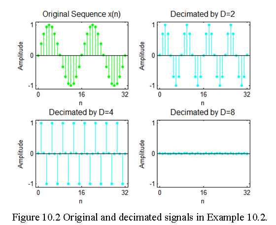
Example 10.2 Let x(n) = sin(0.15\(\pi\) n). Generate a large number of samples of x(n) and decilate them using D = 2, 4, and 8 to show the results of decimation.
% MATLAB Code: n = 0:2048; k1 =256; k2= k1+32; m = 0:(k2-k1);
% (a) Original signal
x = sin(0.125pin); subplot(2,2,1);
Ha = stem(m,x(m+k1+1), ‘g’, ‘filled’); axis([-1,33,-1.1,1.1]);
set(Ha,‘markersize’,2); ylabel(‘Amplitude’);
title(‘Original Sequence x(n)’,‘fontsize’,12);
set(gca,‘xtick’,[0,16,32]); set(gca,‘ytick’,[-1,0,1]);
xlabel(‘n’);
% (b) Decimation by D = 2
D = 2; y = decimate(x,D); subplot(2,2,2);
Hb = stem(m,y(m+k1/D+1), ‘c’, ‘filled’);
axis([-1,33,-1.1,1.1]);
set(Hb,‘markersize’,2); ylabel(‘Amplitude’);
title(‘Decimated by D=2’,‘fontsize’,12);
set(gca,‘xtick’,[0,16,32]); set(gca,‘ytick’,[-1,0,1]);
xlabel(‘n’);
% (c) Decimation by D = 2
D = 4; y = decimate(x,D); subplot(2,2,3);
Hb = stem(m,y(m+k1/D+1), ‘c’, ‘filled’);
axis([-1,33,-1.1,1.1]);
set(Hb,‘markersize’,2); ylabel(‘Amplitude’);
title(‘Decimated by D=4’,‘fontsize’,12);
set(gca,‘xtick’,[0,16,32]); set(gca,‘ytick’,[-1,0,1]);
xlabel(‘n’);
% (d) Decimation by D = 2
D = 8; y = decimate(x,D); subplot(2,2,4);
Hb = stem(m,y(m+k1/D+1), ‘c’, ‘filled’);
axis([-1,33,-1.1,1.1]);
set(Hb,‘markersize’,2); ylabel(‘Amplitude’);
title(‘Decimated by D=8’,‘fontsize’,12);
set(gca,‘xtick’,[0,16,32]); set(gca,‘ytick’,[-1,0,1]);
xlabel(‘n’);
10.3 Interpolation by a Factor I
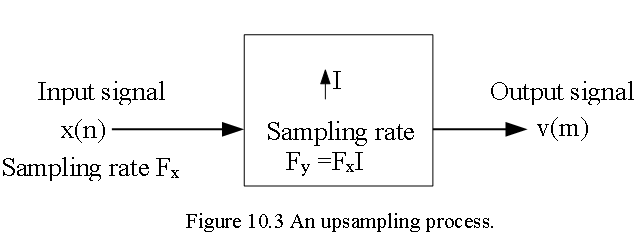
An increase in the sampling rate by an integer factor I is \(F_y = IF_x\) can be found by interpolating \(I-1\) new samples between successive values of the signal. The process of interpolation can be accomplished in two steps. The first step creates an intermediate signal at the high rate \(F_y\) by interlacing zeros in between nonzero samples in an operation called upsampling. In the second step, the intermediate signal is filtered to “fill in” zero-interlaced samples to create the interpolated high-rate signal.
10.3.1 The Upsampler
Let \(v(m)\) enote the intermediate sequence with a rate \(F_y = IF_x\), which is obtained from \(x(n)\) by adding I-1 zeros between successive values of \(x(n)\). Thus
\[\begin{equation} v(m)=\begin{cases} x(m/I), m = 0, \pm I, \pm 2I,....\\ \\ 0, otherwise \end{cases} \tag{10.2} \end{equation}\]
and its sampling rate is identical to the rate of v(m). The block diagram of the upsampler is shown in Figure 10.2. The upsampler is a time-varying system.
Example 10.3 Let I = 2 and \(x(n) = { 2_{\uparrow},5,9,10}\). Verify that the upsampler is time varying.
Solution: The upsampled signal is \(x(n) = { 2_{\uparrow},0,5,0,9,0,10,0}\). If we now delay x(n) by one sample, we get \(x(n-1) = { 0_{\uparrow},2,5,9,10}\)}. The corresponding upsampled signal is \(v_1(m)\)=\({ 0_{\uparrow},0,2,0,5,0,9,0,10,0}=v(m-2)\) and not v(m-1).
% Matlab Implementation
x = [2,5,9,10]; v = upsample(x,2)
v =
2 0 5 0 9 0 10 0x = [2,5,9,10]; v = upsample(x,2,1)
v =
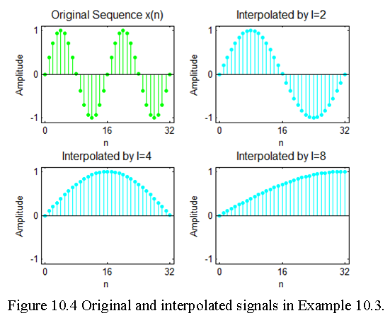
0 2 0 5 0 9 0 10Example 10.4 Let x(n)=cos(\(\pi\)n). Generate samples of x(n) and interpolate them using I =2, 4, and 8 to show the results of interpolation.
Solution: The plots of Figure 10.4 show the middle segments of the signals to avoid end-effects due to the default lowpass filter in the interp function.
% MATLAB Code:
n = 0:256; k1 =64; k2= k1+32; m = 0:(k2-k1);
% (a) Original signal
x = cos(pi*n); subplot(2,2,1);
Ha = stem(m,x(m+k1+1), ‘g’, ‘filled’); axis([-1,33,-1.1,1.1]);
set(Ha,‘markersize’,2); ylabel(‘Amplitude’);
title(‘Original Sequence x(n)’,‘fontsize’,12);
set(gca,‘xtick’,[0,16,32]); set(gca,‘ytick’,[-1,0,1]);
xlabel(‘n’);
% (b) Interpolation by I = 2
I = 2; y = interp(x,I); subplot(2,2,2);
Hb = stem(m,y(m+k1*I+1), ‘c’, ‘filled’);
axis([-1,33,-1.1,1.1]);
set(Hb,‘markersize’,2); ylabel(‘Amplitude’);
title(‘Interpolated by I=2’,‘fontsize’,12);
set(gca,‘xtick’,[0,16,32]); set(gca,‘ytick’,[-1,0,1]);
xlabel(‘n’);
% (c) Interpolation by I = 4
I = 2; y = interp(x,I); subplot(2,2,2);
Hb = stem(m,y(m+k1*I+1), ‘c’, ‘filled’);
axis([-1,33,-1.1,1.1]);
set(Hb,‘markersize’,2); ylabel(‘Amplitude’);
title(‘Interpolated by I=4’,‘fontsize’,12);
set(gca,‘xtick’,[0,16,32]); set(gca,‘ytick’,[-1,0,1]);
xlabel(‘n’);
% (d) Interpolation by I = 8
I = 2; y = interp(x,I); subplot(2,2,2);
Hb = stem(m,y(m+k1*I+1), ‘c’, ‘filled’);
axis([-1,33,-1.1,1.1]);
set(Hb,‘markersize’,2); ylabel(‘Amplitude’);
title(‘Interpolated by I=8’,‘fontsize’,12);
set(gca,‘xtick’,[0,16,32]); set(gca,‘ytick’,[-1,0,1]);
xlabel(‘n’);
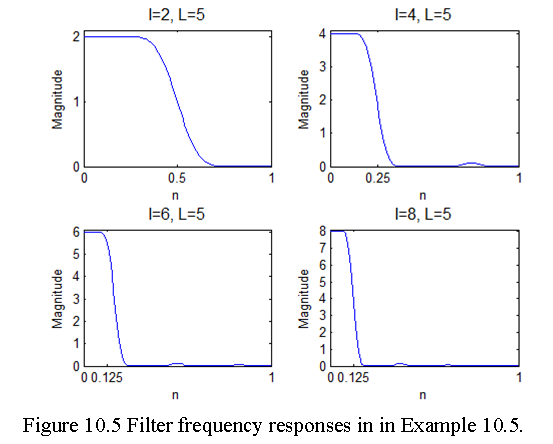
Example 10.5 Examine the frequency response of the lowpass filter used in the interpolation of the signal in Example 10.5.
Solution: The second optional argument in the interp function provides the impulse response from which we can compute the frequency response, as shown in the following Matlab code.
n = 0:256; x = cos(pin); w = [0:100]pi/100;
% (a) Interpolation by I = 2, L =5;
I = 2;L=5; [y,h] = interp(x,I,L); H = freqz(h,1,w); H = abs(H);
subplot(2,2,1); plot(w/pi,H,‘b’); axis([0,1,0,I+0.1]);
ylabel(‘Magnitude’);
title(‘I=2, L=5’,‘fontsize’,12);
set(gca,‘xtick’,[0,0.5,1]); set(gca,‘ytick’,[0:1:I]);
xlabel(‘n’);
% (b) Interpolation by I = 4, L =5;
I = 4; L =5; [y,h] = interp(x,I,L); H = freqz(h,1,w); H = abs(H);
subplot(2,2,2); plot(w/pi,H,‘b’); axis([0,1,0,I+0.1]);
ylabel(‘Magnitude’);
title(‘I=4, L=5’,‘fontsize’,12);
set(gca,‘xtick’,[0,0.25,1]); set(gca,‘ytick’,[0:1:I]);
xlabel(‘n’);
% (c) Interpolation by I = 8, L =5;
I = 6; L =5; [y,h] = interp(x,I,L); H = freqz(h,1,w); H = abs(H);
subplot(2,2,3); plot(w/pi,H,‘b’); axis([0,1,0,I+0.1]);
ylabel(‘Magnitude’);
title(‘I=6, L=5’,‘fontsize’,12);
set(gca,‘xtick’,[0,0.125,1]); set(gca,‘ytick’,[0:1:I]);
xlabel(‘n’);
% (d) Interpolation by I = 8, L =10;
I = 8; L=5; [y,h] = interp(x,I,L); H = freqz(h,1,w); H = abs(H);
subplot(2,2,4); plot(w/pi,H,‘b’); axis([0,1,0,I+0.1]);
ylabel(‘Magnitude’);
title(‘I=8, L=5’,‘fontsize’,12);
set(gca,‘xtick’,[0,0.125,1]); set(gca,‘ytick’,[0:1:I]);
xlabel(‘n’);
10.4 Sampling Rate Conversion by a Rational Factor I/D
In sections 10.2 an 10.3, we discussed the special cases of decimation (downsampling by a factor D) and interpolation (upsampling by a factor I), we now consider the general case of sampling rate conversion by a rational factor I/D. In the I/D conversion, the sampling rate conversion is done by first performing the interpolation by the factor I and then decimation of the output of the interpolator by the factor as illustrated in Figure 10.6.
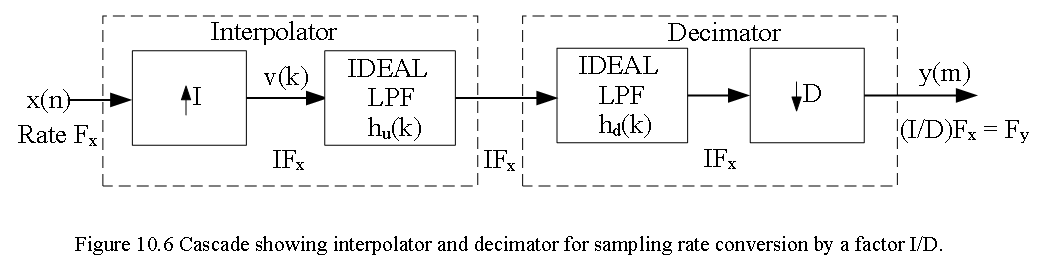
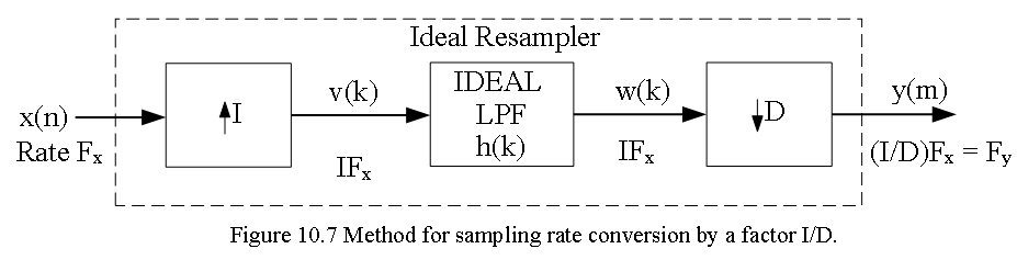
The reason of performing the interpolation first and the decimation second is to keep the desired spectral characteristics of x(n). The cascade configuration as shown in Figure 10.6 with two filters having impulse response \({h_u(k)}\) and \({h_d(k)}\) respectively with same sampling rate \(IF_x\). In Figure 10.7 demonstrated use of one single lowpass filter with impulse response h(k). The frequency response \(H(\omega_v)\) of the combined filter must incorporate the filtering operations for both interpolation and decimation, and hence it should ideally possess the frequency-response characteristic
\[\begin{equation} H(\omega_v)=\begin{cases} I, 0 \le |\omega_v| \le min(\pi/D,\pi /I)\\ \\ 0, otherwise \end{cases} \tag{10.3} \end{equation}\]
where \(\omega_v = \frac{2\pi F}{F_v}=\frac{2\pi F}{IF_x}=\frac{\omega_x}{I}\).
Explanation of Eq. (10.3). Note that \(V(\omega_v)\) and hence \(W(\omega_v)\) in Figure 10.7 are periodic with period \(2\pi/I\). Thus
if D < I, then filter \(H(\omega_v)\) allows a full period through and there is no net lowpass filtering.
if D > I, then filter must first truncate the fundamental period of \(W(\omega_v)\) to avoid aliasing error in the \((D\downarrow 1)\) decimation stage to follow.
Putting these two conditions together, we can observe that when D/I < 1, we have net interpolation and no smoothing is required by \(H(\omega_v)\) other than to extract the fundamental period of \(W(\omega_v)\). In this respect, \(H(\omega_v)\) acts as a lowpass filter as in the ideal interpolator. On the other hand, if D/I > 1, then we have net decimation. Therefore, it is necessary to first truncate even the fundamental period of \(W(\omega_v)\) to get the frequency band down to [-/D, /D] and to avoid aliasing in the decimation that follows. In this respect, \(H(\omega_v)\) acts as a smoothing filter in the ideal decimator.
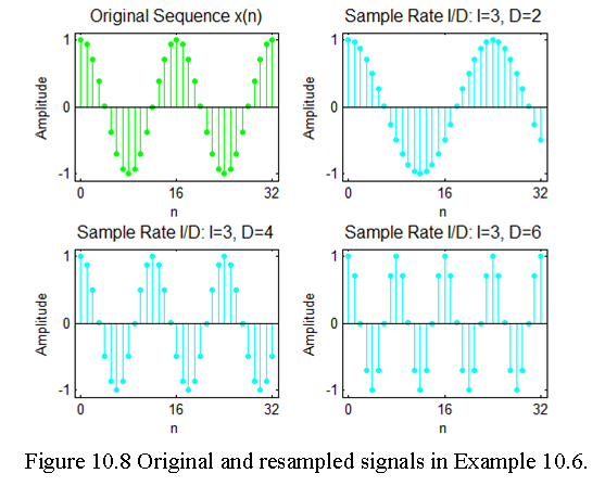
Example 10.6 Consider the sequence x(n) = cos(0.125\(\pi\) n) as discussed in Example 10-2, with the change in the sampling rate to 3/2, 3/4, and 5/8.
The following MATLAB code performs the required implementation:
n = 0:2048; k1 = 256; k2 = k1+32; m = 0:(k2-k1);
% (a) Original signal
x = cos(0.125pin); subplot(2,2,1);
Ha = stem(m,x(m+k1+1), ‘g’, ‘filled’); axis([-1,33,-1.1,1.1]);
set(Ha,‘markersize’,2); ylabel(‘Amplitude’);
title(‘Original Sequence x(n)’,‘fontsize’,12);
set(gca,‘xtick’,[0,16,32]); set(gca,‘ytick’,[-1,0,1]);
xlabel(‘n’);
% (b) Sample conversion rate by 3/2; I =3, D =2
I = 3;D=2; y = resample(x,I,D); subplot(2,2,2);
Hb = stem(m,y(m+k1*I+1), ‘c’, ‘filled’);
axis([-1,33,-1.1,1.1]);
set(Hb,‘markersize’,2); ylabel(‘Amplitude’);
title(‘Sample Rate I/D: I=3, D=2’,‘fontsize’,12);
set(gca,‘xtick’,[0,16,32]); set(gca,‘ytick’,[-1,0,1]);
xlabel(‘n’);
% (c) Sample conversion rate by 3/2; I =3, D =4
I = 3;D = 4; y = resample(x,I,D);subplot(2,2,3);
Hb = stem(m,y(m+k1*I+1), ‘c’, ‘filled’);
axis([-1,33,-1.1,1.1]);
set(Hb,‘markersize’,2); ylabel(‘Amplitude’);
title(‘Sample Rate I/D: I=3, D=4’,‘fontsize’,12);
set(gca,‘xtick’,[0,16,32]); set(gca,‘ytick’,[-1,0,1]);
xlabel(‘n’);
% (d) Sample conversion rate by 3/2; I =5, D =8
I = 3;D = 6; y = resample(x,I,D);subplot(2,2,4);
Hb = stem(m,y(m+k1*I+1), ‘c’, ‘filled’);
axis([-1,33,-1.1,1.1]);
set(Hb,‘markersize’,2); ylabel(‘Amplitude’);
title(‘Sample Rate I/D: I=3, D=6’,‘fontsize’,12);
set(gca,‘xtick’,[0,16,32]); set(gca,‘ytick’,[-1,0,1]);
xlabel(‘n’);