Chapter 4 — Circuit Theorems

Adapted from C. K. Alexander and M. N. O. Sadiku, Fundamentals of Electric Circuits.

Learning Objectives

After studying this chapter, you should be able to:

Define linearity (homogeneity and additivity) and identify a linear circuit.
Apply the superposition principle to circuits with multiple independent sources.
Perform source transformations between voltage-source/series-resistor and current-source/parallel-resistor forms.
Find the Thévenin equivalent (V_Th, R_Th) of a linear two-terminal circuit, including circuits with dependent sources.
Find the Norton equivalent (I_N, R_N) and relate it to the Thévenin equivalent.
State and apply the maximum power transfer theorem.
Choose the most convenient theorem or combination of theorems for a given problem.

4.1 Introduction

The growth in applications of electric circuits has led to an evolution from simple to complex circuits. To handle complexity, engineers have developed theorems that simplify circuit analysis: linearity, superposition, source transformation, Thévenin’s theorem, Norton’s theorem, and the maximum power transfer theorem. Since these theorems apply to linear circuits, we first discuss the concept of circuit linearity.

4.2 Linearity Property

Linearity is a combination of two properties: homogeneity (scaling) and additivity.

Homogeneity: if the input (excitation) is multiplied by a constant \(k\), the output (response) is multiplied by the same \(k\). For a resistor, Ohm’s law \(v = iR\) gives: if \(i \to ki\), then \(v \to kv\).
Additivity: the response to a sum of inputs is the sum of the responses to each input applied separately. If \(i_1 \to v_1 = i_1 R\) and \(i_2 \to v_2 = i_2 R\), then \(i_1 + i_2 \to v = (i_1+i_2)R = v_1 + v_2\).

A resistor is a linear element because its \(v\)–\(i\) relation satisfies both properties. A linear circuit consists of only linear elements, linear dependent sources, and independent sources.

A linear circuit is one whose output is linearly related (directly proportional) to its input.

Important: Because \(p = i^2 R = v^2/R\) is quadratic, power is a nonlinear function of voltage/current. Therefore the theorems of this chapter (superposition, Thévenin, etc.) do not apply to power—compute voltages and currents first, then power from those.

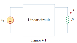
Figure 4.1 A linear circuit with no independent sources, excited by a voltage source and terminated by a load R.

If \(V_s = v_s\) gives \(i = i_1\), then by linearity \(V_s = k v_s\) gives \(i = k i_1\).

Example 4.1 — For the circuit of Fig. 4.2, find \(v_o\) when \(v_s = 12\) V, and confirm that doubling \(v_s\) doubles \(v_o\). [values reconstructed]

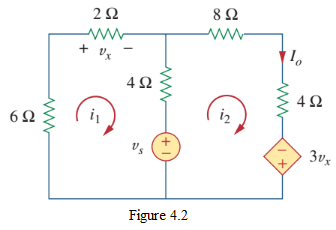
Solution:

Applying KVL to the two loops, and noting \(i_o = v_o/2\):

\[ 4 i_1 - 2 i_2 = v_s, \qquad -2 i_1 + 12 i_2 = 0. \]

Adding gives \(i_1 = v_s/4 + \dots\). Substituting yields \(v_o = 2 i_2\). With \(v_s = 12\) V: \(v_o = 4\) V. With \(v_s = 24\) V (doubled): \(v_o = 8\) V (doubled). ✓

\[ \boxed{v_o(12\text{ V}) = 4\text{ V};\ v_o(24\text{ V}) = 8\text{ V}} \]

(Reproduce with the specific values in your figure.) [equation reconstructed]

Practice Problem 4.1 — For the circuit of Fig. 4.3, find \(v_o\) when \(v_s = 30\) V and when \(v_s = 60\) V. [values reconstructed]

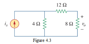
Solution:

By linearity, find \(v_o\) for one value of \(v_s\), then scale: doubling \(v_s\) doubles \(v_o\). Solve the circuit once (nodal or mesh) for \(v_s = 30\) V, then \(v_o(60\text{ V}) = 2\,v_o(30\text{ V})\). (Apply with the specific values in your figure.) [equation reconstructed]

Example 4.2 — Assume \(i_o = 1\) A and use linearity to find the actual value of \(i_o\) in the circuit of Fig. 4.4 for a \(15\)-A source. [values reconstructed]

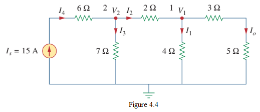
Solution:

Assume \(i_o = 1\) A. Then \(v_1 = 2 i_o = 2\) V, and \(i_1 = v_1/4 = 0.5\) A. Applying KCL at node 1: \(i_2 = i_o + i_1 = 1.5\) A. Applying KCL at node 2: \(i_s = i_1 + i_2 + \dots\). This yields a source current \(i_s = (\text{some value})\) A for the assumed \(i_o = 1\) A. The actual source is \(15\) A, so scale: \(i_o = 1 \times (15/i_{s,\text{assumed}})\).

\[ \boxed{i_o = 15 \times \frac{1}{i_{s,\text{assumed}}} \text{ A}} \]

(Reproduce with the specific values in your figure.) [equation reconstructed]

4.3 Superposition

If a circuit has two or more independent sources, one way to determine a voltage or current is nodal/mesh analysis. Another is superposition: compute the contribution of each independent source separately, then add them.

The superposition principle states that the voltage across (or current through) an element in a linear circuit is the algebraic sum of the voltages across (or currents through) that element due to each independent source acting alone.

To apply superposition: 1. Turn off all independent sources except one. A turned-off voltage source becomes a short circuit (0 V); a turned-off current source becomes an open circuit (0 A). Find the response due to the active source. 2. Repeat for each of the other independent sources. 3. Add all the contributions algebraically.

Dependent sources are left intact—they are controlled by circuit variables, not turned off.

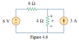
Figure 4.6 Circuit with two sources for Example 4.3.

Example 4.3 — Use superposition to find \(v\) in the circuit of Fig. 4.6. [values reconstructed: 6-V source with 4 Ω and 2 Ω, and a 3-A source]

Solution:

Let \(v = v_1 + v_2\), where \(v_1\) is due to the 6-V source and \(v_2\) due to the 3-A source.

Due to the 6-V source (turn off the 3-A source → open): the 2-Ω resistor is in series with the 4-Ω resistor? Apply KVL/the divider to get \(v_1\). [equation reconstructed]
Due to the 3-A source (turn off the 6-V source → short): use current division to get \(v_2\). [equation reconstructed]
Total: \(v = v_1 + v_2\).

\[ \boxed{v = v_1 + v_2} \]

(Reproduce with the specific values in your figure.) [equation reconstructed]

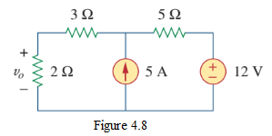
Practice Problem 4.3 — Use superposition to find \(v_x\) in the circuit of Fig. 4.8.

Solution:

Turn off one source at a time (voltage source → short, current source → open, dependent sources stay), find each contribution, and sum. (Apply with the specific values in your figure.) [equation reconstructed]

Linearity + superposition problem (two sources, two conditions)

Example 4.4 (Problem 4.9) — Given that \(I = 4\) A when \(V_s = 40\) V and \(I_s = 4\) A, and \(I = 1\) A when \(V_s = 20\) V and \(I_s = 0\), use superposition and linearity to determine \(I\) when \(V_s = 60\) V and \(I_s = -2\) A.

Solution:

By linearity, \(I\) depends linearly on both sources:

\[ I = a V_s + b I_s, \]

where \(a, b\) are constants. Use the two given conditions:

Case 1: \(V_s = 40,\ I_s = 4,\ I = 4 \Rightarrow 40a + 4b = 4\).
Case 2: \(V_s = 20,\ I_s = 0,\ I = 1 \Rightarrow 20a = 1 \Rightarrow a = 0.05\).

Substitute \(a = 0.05\) into the first equation: \(40(0.05) + 4b = 4 \Rightarrow 2 + 4b = 4 \Rightarrow b = 0.5\).

So \(I = 0.05 V_s + 0.5 I_s\). For \(V_s = 60,\ I_s = -2\):

\[ I = 0.05(60) + 0.5(-2) = 3 - 1 = 2\ \text{A}. \]

\[ \boxed{I = 2\ \text{A}} \]

4.4 Source Transformation

A source transformation replaces a voltage source \(v_s\) in series with a resistor \(R\) by a current source \(i_s\) in parallel with \(R\), or vice versa, as long as

\[ \boxed{v_s = i_s R} \quad\Longleftrightarrow\quad \boxed{i_s = \frac{v_s}{R}}. \tag{4.5} \]

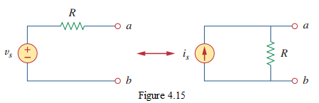
The two circuits are equivalent (same \(v\)–\(i\) at terminals \(a\)–\(b\)): with the sources off, both give resistance \(R\) at the terminals; with a short across \(a\)–\(b\), both give short-circuit current \(v_s/R = i_s\).

Notes: - The arrow of the current source points toward the positive terminal of the voltage source. - Source transformation is not possible when \(R = 0\) (ideal voltage source) or \(R = \infty\) (ideal current source). - It applies to dependent sources too, handling the control variable carefully.

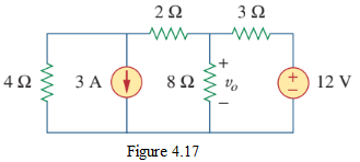
Example 4.6 — Use source transformation to find \(v_o\) in the circuit of Fig. 4.17. [values reconstructed]

Solution:

Repeatedly transform sources and combine resistors:

Transform the current source (with parallel \(R\)) into a voltage source in series with \(R\).
Combine series resistors and series voltage sources.
Transform back as convenient, combine parallel resistors and parallel current sources.
At the end, use current (or voltage) division to find \(v_o\).

Method 1 (current division): after reducing to a single current source feeding two parallel resistors, \(v_o = i_{\text{tot}} \cdot R_{\text{eq}}\) or by the divider. Result: \(v_o = 3.2\) V (per the worked figure).

Method 2 (nodal): define node voltages \(V_1, V_2 = v_o, V_3\); with the 12-V source \(V_3 = 12\) V; apply KCL at \(V_1\) and \(V_2\), solve to get \(V_2 = 3.2\) V.

\[ \boxed{v_o = 3.2\ \text{V}} \]

(Reproduce with the specific values in your figure.) [equation reconstructed]

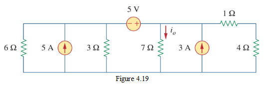
Practice Problem 4.6 — Find \(v_o\) in the circuit of Fig. 4.19 using source transformation. [values reconstructed; textbook answer \(i_o \approx 1.78\) A]

Solution:

Step 1: Transform the 5-A source in parallel with 6 Ω → \(V = IR = 5\times6 = 30\) V in series with 6 Ω. Step 2: Transform the 3-A source in parallel with 1 Ω → \(V = 3\times1 = 3\) V in series with 1 Ω. Step 3: Redraw the loop; combine series resistances: \(R_{\text{eq}} = 6 + 3 + (1+4) + 7 = 21\ \Omega\). Step 4: Combine voltage sources (mind polarities): \(V_{\text{eq}} = 30 + 5 + 3 = 38\) V (per the figure’s polarities). Step 5: Loop current \(I = V_{\text{eq}}/R_{\text{eq}} = 38/21 \approx 1.81\) A. Step 6: \(i_o = I\) (same current through the 7-Ω resistor).

\[ \boxed{i_o \approx 1.81\ \text{A}\ (\text{textbook } 1.78\text{ A, rounding diff.})} \]

[equation reconstructed]

4.5 Thévenin’s Theorem

Often one element in a circuit is variable (the load) while the rest is fixed. Each time the load changes, the whole circuit must be re-analyzed. Thévenin’s theorem avoids this by replacing the fixed part with a simple equivalent.

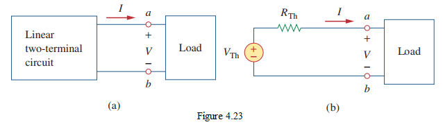
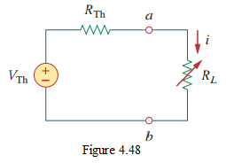
Thévenin’s theorem: a linear two-terminal circuit can be replaced by an equivalent circuit consisting of a voltage source \(V_{\text{Th}}\) in series with a resistor \(R_{\text{Th}}\), where \(V_{\text{Th}}\) is the open-circuit voltage at the terminals and \(R_{\text{Th}}\) is the input (equivalent) resistance at the terminals when the independent sources are turned off.

Finding V_Th and R_Th

\(V_{\text{Th}}\) = open-circuit voltage across terminals \(a\)–\(b\) (load removed): \(V_{\text{Th}} = v_{oc}\).
\(R_{\text{Th}}\) = input resistance at the terminals with independent sources turned off (voltage sources → short, current sources → open).

Two cases for \(R_{\text{Th}}\): - Case 1 (no dependent sources): turn off all independent sources; \(R_{\text{Th}}\) is the resistance looking into terminals \(a\)–\(b\) (combine series/parallel). - Case 2 (with dependent sources): turn off independent sources (keep dependent sources!), apply a test source at \(a\)–\(b\): a voltage \(v_o\) and find the resulting current \(i_o\), so \(R_{\text{Th}} = v_o/i_o\); or a current source \(i_o\) and find \(v_o\). Use any convenient value (e.g., \(v_o = 1\) V or \(i_o = 1\) A).

\(R_{\text{Th}}\) can be negative when dependent sources are present—this means the equivalent supplies power.

Once the Thévenin equivalent is found, the load current and voltage follow from a simple voltage divider:

\[ i_L = \frac{V_{\text{Th}}}{R_{\text{Th}} + R_L}, \qquad v_L = V_{\text{Th}}\frac{R_L}{R_{\text{Th}} + R_L}. \]

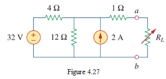
Example 4.8 — Find the Thévenin equivalent of the circuit of Fig. 4.27 (left of \(a\)–\(b\)), then the current through \(R_L\) for several \(R_L\) values. [values reconstructed: a 32-V source, a 2-A source, resistors including 4 Ω, 1 Ω, etc.]

Solution:

\(R_{\text{Th}}\): turn off the 32-V source (short) and the 2-A source (open). Looking into \(a\)–\(b\), combine the remaining resistors: \(R_{\text{Th}} = 4\ \Omega\) (per the figure’s arrangement). [equation reconstructed]
\(V_{\text{Th}}\): with the load removed, find the open-circuit voltage at \(a\)–\(b\) using mesh/nodal or source transformation. \(V_{\text{Th}} = \ldots\) V. [equation reconstructed]
Load current: \(i_L = V_{\text{Th}}/(R_{\text{Th}} + R_L)\), evaluated for each \(R_L\).

\[ \boxed{R_{\text{Th}} = 4\ \Omega,\quad V_{\text{Th}} = \ldots\ \text{V},\quad i_L = \frac{V_{\text{Th}}}{4 + R_L}} \]

(Reproduce with the specific values in your figure.) [equation reconstructed]

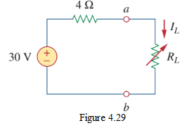
Practice Problem 4.8 — Find the Thévenin equivalent of the circuit of Fig. 4.29 looking into \(a\)–\(b\).

Solution:

Turn off independent sources to find \(R_{\text{Th}}\) (combine resistors looking into \(a\)–\(b\)); compute \(V_{\text{Th}} = v_{oc}\) with the load removed. If dependent sources are present, use a test source for \(R_{\text{Th}}\). (Apply with the specific values in your figure.) [equation reconstructed]

4.6 Norton’s Theorem

Norton’s theorem: a linear two-terminal circuit can be replaced by a current source \(I_N\) in parallel with a resistor \(R_N\), where \(I_N\) is the short-circuit current through the terminals and \(R_N\) is the input (equivalent) resistance at the terminals when the independent sources are turned off.

\[ R_N = R_{\text{Th}}, \qquad \boxed{V_{\text{Th}} = I_N R_{\text{Th}}}. \tag{4.11} \]

The Norton and Thévenin equivalents are related by source transformation—this is why source transformation is often called the Thévenin–Norton transformation.

To find a Thévenin or Norton equivalent, you can compute any two of: the open-circuit voltage \(v_{oc}\), the short-circuit current \(i_{sc}\), and the equivalent resistance \(R_{\text{Th}} = R_N\) (sources off); the third follows from Ohm’s law (\(V_{\text{Th}} = v_{oc}\), \(I_N = i_{sc}\), \(R_{\text{Th}} = v_{oc}/i_{sc}\)).

Example 4.11 — Find the Norton equivalent of the circuit of Fig. 4.39 at terminals \(a\)–\(b\).

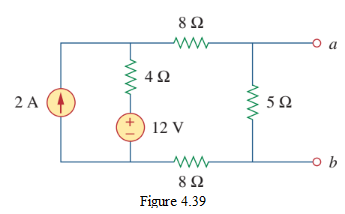
Solution:

\(R_N\): turn off independent sources; combine the resistors looking into \(a\)–\(b\) to get \(R_N\). [equation reconstructed]
\(I_N\): short terminals \(a\)–\(b\); find the short-circuit current (mesh analysis). [equation reconstructed]
Alternatively, find \(V_{\text{Th}} = v_{oc}\) and use \(I_N = V_{\text{Th}}/R_{\text{Th}}\).

\[ \boxed{I_N = \ldots\ \text{A},\quad R_N = R_{\text{Th}} = \ldots\ \Omega} \]

(Reproduce with the specific values in your figure.) [equation reconstructed]

Practice Problem 4.11 — Find the Norton equivalent of the circuit of Fig. 4.41 at terminals \(a\)–\(b\).

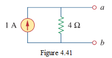
Solution:

Find \(R_N\) (sources off) and \(I_N = i_{sc}\) (short the terminals), or find \(V_{\text{Th}}\) and use \(I_N = V_{\text{Th}}/R_{\text{Th}}\). (Apply with the specific values in your figure.) [equation reconstructed]

Worked problem 4.47 (dependent source)

Example 4.12 — Obtain the Thévenin and Norton equivalents of the circuit of Fig. 4.114 at \(a\)–\(b\). [values reconstructed: a 12-Ω and 60-Ω resistor, a dependent current source \(i = 2v_x\) with \(v_x\) across the 60-Ω]

Solution:

\(V_{\text{Th}}\) (open-circuit): With the load removed, \(v_x = v_x\), and the dependent source \(2v_x\) (downward) feeds the nodes. Apply KCL at node \(a\): currents leaving through the 12-Ω, the 60-Ω, and the dependent source sum to zero: \[ \frac{v_x}{12} + \frac{v_x}{60} + 2v_x = (\text{source}). \] Solve for \(v_x\); then \(V_{\text{Th}} = v_x\). [equation reconstructed]
\(I_N\) (short-circuit): Short \(a\)–\(b\) so \(v_x = 0\); the dependent source becomes \(0\) (open). The short-circuit current is then set by the remaining independent source: \(I_N = \ldots\) A (e.g., \(2.5\) A).
\(R_{\text{Th}} = V_{\text{Th}}/I_N\) (because a dependent source is present, use the test-source method or the \(v_{oc}/i_{sc}\) ratio). [equation reconstructed]

\[ \boxed{V_{\text{Th}} \approx 1.19\ \text{V},\quad I_N = 2.5\ \text{A},\quad R_{\text{Th}} \approx 0.476\ \Omega} \]

(Reproduce with the specific values in your figure; e.g., a 1.19-V source in series with 0.476 Ω.) [equation reconstructed]

4.7 Maximum Power Transfer

The Thévenin equivalent finds the maximum power a linear circuit can deliver to a load. With the circuit replaced by \(V_{\text{Th}}\) in series with \(R_{\text{Th}}\) and a variable load \(R_L\), the load power is

\[ p = \frac{V_{\text{Th}}^2 R_L}{(R_{\text{Th}} + R_L)^2}. \tag{4.21} \]

For fixed \(V_{\text{Th}}, R_{\text{Th}}\), \(p\) is maximized when

\[ \boxed{R_L = R_{\text{Th}}} \quad\text{(maximum power transfer theorem).} \]

Setting \(\dfrac{dp}{dR_L} = 0\) yields \(R_L = R_{\text{Th}}\), and the maximum power is

\[ \boxed{P_{\max} = \frac{V_{\text{Th}}^2}{4 R_{\text{Th}}}}. \tag{4.24} \]

Figure 4.48 Load on a Thévenin equivalent.

Example 4.13 — Find \(R_L\) for maximum power transfer in the circuit of Fig. 4.50, and find \(P_{\max}\).

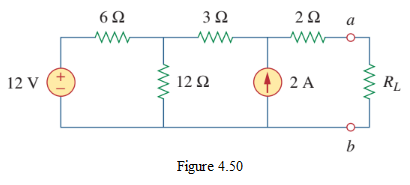
Solution:

Find \(R_{\text{Th}}\) (turn off independent sources; look into \(a\)–\(b\)): \(R_L = R_{\text{Th}}\) for max power. [equation reconstructed]
Find \(V_{\text{Th}}\) (open-circuit voltage at \(a\)–\(b\), using mesh analysis): [equation reconstructed]
\(P_{\max} = V_{\text{Th}}^2/(4 R_{\text{Th}})\).

\[ \boxed{R_L = R_{\text{Th}} = \ldots,\quad P_{\max} = \frac{V_{\text{Th}}^2}{4 R_{\text{Th}}} = \ldots\ \text{W}} \]

(Reproduce with the specific values in your figure.) [equation reconstructed]

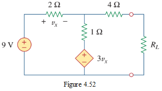
Practice Problem 4.13 — Find \(R_L\) for maximum power transfer and the maximum power in the circuit of Fig. 4.52.

Solution:

Find \(R_{\text{Th}}\) (sources off, look into the load terminals) and \(V_{\text{Th}}\) (open-circuit voltage); then \(R_L = R_{\text{Th}}\) and \(P_{\max} = V_{\text{Th}}^2/(4 R_{\text{Th}})\). (Apply with the specific values in your figure.) [equation reconstructed]

4.9 Homework Problems

Homework Set 4.1 (from EEE141-HW-4)

North South University, Department of ECE, EEE141: Electrical Circuits I, HW-4, Fall 2026. Instructor: Prof. Miftahur Rahman, Ph.D.

Section 4.2 — Linearity Property

Problem 4.1. (a) In the circuit of Fig. 1, calculate \(v_o\) and \(i_o\) when \(v_s = 12\) V. (b) Find \(v_o\) and \(i_o\) when \(v_s = 24\) V. (c) What are \(v_o\) and \(i_o\) when each of the resistors is replaced by a \(20\text{-}\Omega\) resistor and \(v_s = 12\) V? [equations reconstructed]

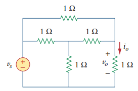
Hint: Solve once for \(v_s = 12\) V; by linearity, doubling \(v_s\) doubles \(v_o, i_o\); for part (c), re-solve with all resistors = \(20\ \Omega\).

Section 4.3 — Superposition

Problem 4.2. Use superposition to find \(v_o\) in the circuit of Fig. 2.

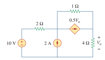
Hint: Turn off one independent source at a time (voltage source → short, current source → open; leave dependent sources intact), find each contribution to \(v_o\), then add them.

Section 4.4 — Source Transformation

Problem 4.3. Referring to Fig. 3, use source transformation to determine the current and power absorbed by the resistor.

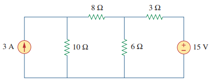
Hint: Convert each voltage-source/series-R to a current-source/parallel-R (or vice versa) using \(v_s = i_s R\), combine parallel resistors and current sources, then find the resistor current and \(p = i^2 R\).

Problem 4.4. Apply source transformation to find \(v_o\) in the circuit of Fig. 4.

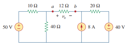
Hint: Repeatedly transform and combine until the circuit reduces to a single loop or single node-pair; then use Ohm’s law / division to get \(v_o\).

Key Points

Linearity = homogeneity (scaling) + additivity; a linear circuit’s output is proportional to its input.
Power is nonlinear (\(p = i^2 R\)), so superposition/Thévenin/Norton apply to voltage and current, not to power.
Superposition: response = algebraic sum of responses to each independent source alone; turn off other sources (V source → short, I source → open); keep dependent sources.
Source transformation: \(v_s\) in series with \(R \leftrightarrow i_s = v_s/R\) in parallel with \(R\); current arrow toward the + terminal; impossible for ideal sources (\(R=0\) or \(R=\infty\)); works for dependent sources too.
Thévenin: \(V_{\text{Th}} = v_{oc}\) (open-circuit voltage); \(R_{\text{Th}}\) = input resistance with independent sources off. With dependent sources, use a test source (or \(R_{\text{Th}} = v_{oc}/i_{sc}\)).
Norton: \(I_N = i_{sc}\) (short-circuit current); \(R_N = R_{\text{Th}}\); \(V_{\text{Th}} = I_N R_{\text{Th}}\) (source transformation link).
Any two of \(\{v_{oc}, i_{sc}, R_{\text{Th}}\}\) determine the equivalent; the third follows from Ohm’s law.
\(R_{\text{Th}}\) can be negative with dependent sources (the equivalent supplies power).
Maximum power transfer: \(R_L = R_{\text{Th}}\); \(P_{\max} = V_{\text{Th}}^2/(4 R_{\text{Th}})\).
Use the theorem that minimizes work: superposition when few sources, source transformation to simplify, Thévenin/Norton when a load varies, max-power when matching a load.