Chapter 2 — Basic Laws
Adapted from C. K. Alexander and M. N. O. Sadiku, Fundamentals of Electric Circuits.
Learning Objectives
After studying this chapter, you should be able to:
- State and apply Ohm’s law (\(v = iR\)) and relate resistance to resistivity, length, and cross-sectional area.
- Distinguish short circuits, open circuits, fixed and variable resistors, and linear vs nonlinear resistors.
- Define and use conductance \(G = 1/R\) (siemens) and express resistor power in terms of \(R\) or \(G\).
- Define branch, node, and loop and identify series and parallel connections.
- State and apply Kirchhoff’s current law (KCL) and Kirchhoff’s voltage law (KVL), including combining sources in parallel and series.
- Combine series and parallel resistors into equivalent resistances.
- Apply voltage division and current division.
- Perform wye–delta (Y–Δ) and delta–wye (Δ–Y) transformations.
2.1 Introduction
Chapter 1 introduced the basic concepts of current, voltage, and power. In this chapter we establish the fundamental laws—Ohm’s law and Kirchhoff’s laws—on which all electric circuit analysis is built. We then develop the essential techniques that follow from them: combining resistors in series and parallel, voltage division, current division, and the wye–delta (Y–Δ) transformations. Together with the methods of Chapter 3 and the theorems of Chapter 4, these tools let us analyze essentially any linear DC circuit.
2.2 Ohm’s Law
The ability to resist current is known as resistance, represented by the symbol \(R\). The resistance of any material with a uniform cross-sectional area \(A\) depends on \(A\) and its length \(\ell\), as shown in Fig. 2.1:
\[ R = \rho \frac{\ell}{A} \tag{2.1} \]
where \(\rho\) is the resistivity of the material in ohm-meters (\(\Omega\cdot\text{m}\)). Good conductors such as copper and aluminum have low resistivities, while insulators such as mica and paper have high resistivities.
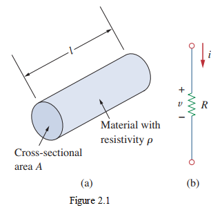
Ohm’s law states that the voltage \(v\) across a resistor is directly proportional to the current \(i\) flowing through the resistor:
\[ v \propto i. \]
Ohm defined the constant of proportionality to be the resistance \(R\). Thus,
\[ \boxed{v = iR} \tag{2.3} \]
which is the mathematical form of Ohm’s law. \(R\) is measured in ohms (\(\Omega\)), where
\[ 1\ \Omega = 1\ \text{V/A}. \]
From Eq. (2.3),
\[ i = \frac{v}{R}, \qquad R = \frac{v}{i}. \tag{2.4} \]
The direction of current \(i\) and the polarity of voltage \(v\) must conform to the passive sign convention: current flows from a higher potential to a lower potential so that \(v = iR > 0\). If current flows from a lower to a higher potential, \(v = -iR\).
Short and open circuits
For a short circuit, \(R = 0\):
\[ v = iR = 0, \tag{2.5} \]
showing the voltage is zero but the current could be anything. A short circuit is a circuit element with resistance approaching zero—typically a connecting wire assumed to be a perfect conductor.
For an open circuit, \(R \to \infty\):
\[ i = \frac{v}{R} = 0, \tag{2.6} \]
indicating the current is zero though the voltage could be anything. An open circuit is a circuit element with resistance approaching infinity.
Resistor types
A resistor is either fixed or variable. Most resistors are fixed—their resistance is constant. The two common types of fixed resistors are wire-wound and composition:
| Feature | Wire-Wound Resistor | Composition Resistor |
|---|---|---|
| Material | Nichrome / Manganin wire | Carbon + binder |
| Core | Ceramic / Porcelain | Solid molded body |
| Power rating | High | Low to medium |
| Accuracy | High | Low |
| Noise | Very low | High |
| Frequency use | Poor (inductive) | Good |
| Cost | Higher | Lower |
A wire-wound resistor is made by winding a resistive metal wire around an insulating core; its resistance depends on the length, diameter, and material of the wire. A composition resistor is made by mixing resistive materials with a binder and molding them into shape.
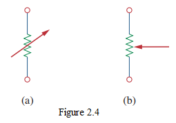
The symbol for a variable resistor is shown in Fig. 2.4(a). A common variable resistor is the potentiometer (pot), a three-terminal element with a sliding contact or wiper, shown in Fig. 2.4(b).
Linear and nonlinear resistors
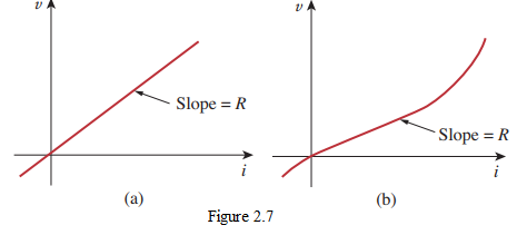
A resistor that obeys Ohm’s law is a linear resistor: it has constant resistance and its \(i\)–\(v\) characteristic is a straight line through the origin. A nonlinear resistor does not obey Ohm’s law; its resistance varies with current and its \(i\)–\(v\) characteristic is curved. Examples of nonlinear devices are the light bulb and the diode.
Conductance
A useful quantity is the reciprocal of resistance, called conductance \(G\):
\[ G = \frac{1}{R} = \frac{i}{v}. \tag{2.7} \]
The unit of conductance is the siemens (S):
\[ 1\ \text{S} = 1\ \text{A/V}. \tag{2.8} \]
For example, \(10\ \Omega\) is the same as \(0.1\ \text{S}\). From Eq. (2.7),
\[ i = vG. \tag{2.9} \]
The power dissipated by a resistor can be expressed in terms of \(R\) (using \(p = vi = (iR)i\)):
\[ p = i^2 R = \frac{v^2}{R}, \tag{2.10} \]
or in terms of \(G\):
\[ p = v^2 G = \frac{i^2}{G}. \tag{2.11} \]
Two observations: (1) the power dissipated in a resistor is a nonlinear function of current or voltage; (2) since \(R\) and \(G\) are positive, the power dissipated is always positive—so a resistor always absorbs power. This confirms a resistor is a passive element, incapable of generating energy.
Example 2.1 — An electric iron draws 2 A at 120 V. Find its resistance.
Solution:
From Ohm’s law,
\[ R = \frac{v}{i} = \frac{120\ \text{V}}{2\ \text{A}} = 60\ \Omega. \]
\[ \boxed{R = 60\ \Omega} \]
Practice Problem 2.1 — The essential component of a toaster is an electrical element (a resistor) that converts electrical energy to heat energy. How much current is drawn by a toaster with resistance \(15\ \Omega\) at \(110\) V?
Solution:
\[ i = \frac{v}{R} = \frac{110\ \text{V}}{15\ \Omega} = 7.333\ \text{A}. \]
\[ \boxed{i \approx 7.33\ \text{A}} \]
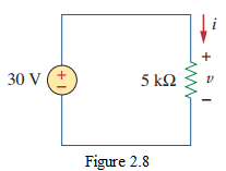
Example 2.2 — In the circuit of Fig. 2.8, calculate the current \(i\), the conductance \(G\), and the power \(p\). The source is \(30\) V across a \(5\ \Omega\) resistor. [values reconstructed]
Solution:
The voltage across the resistor equals the source voltage (30 V) because the resistor and source share the same pair of terminals. Hence the current is
\[ i = \frac{v}{R} = \frac{30}{5} = 6\ \text{A}. \]
The conductance is
\[ G = \frac{1}{R} = \frac{1}{5} = 0.2\ \text{S}. \]
The power can be computed three ways:
\[ p = vi = (30)(6) = 180\ \text{W}, \quad p = i^2 R = (6)^2(5) = 180\ \text{W}, \quad p = \frac{v^2}{R} = \frac{30^2}{5} = 180\ \text{W}. \]
\[ \boxed{i = 6\ \text{A},\quad G = 0.2\ \text{S},\quad p = 180\ \text{W}} \]
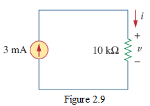
Practice Problem 2.2 — For the circuit of Fig. 2.9 (a \(20\) V source across an \(8\ \Omega\) resistor), calculate the voltage \(v\), the conductance \(G\), and the power \(p\). [values reconstructed]
Solution:
\[ i = \frac{20}{8} = 2.5\ \text{A}, \qquad G = \frac{1}{8} = 0.125\ \text{S}, \qquad p = \frac{20^2}{8} = 50\ \text{W}. \]
\[ \boxed{v = 20\ \text{V},\quad G = 0.125\ \text{S},\quad p = 50\ \text{W}} \]
Example 2.3 — A voltage source of \(v_s = 30\) V is connected across a \(5\text{-k}\Omega\) resistor. Find the current through the resistor and the power dissipated. [values reconstructed]
Solution:
\[ i = \frac{v_s}{R} = \frac{30\ \text{V}}{5\times10^{3}\ \Omega} = 6\times10^{-3}\ \text{A} = 6\ \text{mA}. \]
\[ p = \frac{v_s^2}{R} = \frac{(30)^2}{5\times10^{3}} = \frac{900}{5000} = 0.18\ \text{W} = 180\ \text{mW}. \]
\[ \boxed{i = 6\ \text{mA},\quad p = 180\ \text{mW}} \]
Practice Problem 2.3 — A resistor absorbs an instantaneous power of \(120\) mW when connected to a voltage source \(v = 12\) V. Find \(i\) and \(R\). [values reconstructed]
Solution:
\[ i = \frac{p}{v} = \frac{120\times10^{-3}}{12} = 10\ \text{mA}, \qquad R = \frac{v}{i} = \frac{12}{10\times10^{-3}} = 1200\ \Omega = 1.2\ \text{k}\Omega. \]
\[ \boxed{i = 10\ \text{mA},\quad R = 1.2\ \text{k}\Omega} \]
2.3 Nodes, Branches, and Loops
A branch represents a single element such as a voltage source or a resistor—i.e., any two-terminal element. The circuit in Fig. 2.10 has five branches: the \(10\)-V voltage source, the \(2\)-A current source, and three resistors.
A node is the point of connection between two or more branches. A node is usually indicated by a dot. The circuit in Fig. 2.10 has three nodes \(a\), \(b\), and \(c\). The points connected by perfect conductors constitute a single node even if drawn spread out.
A loop is any closed path in a circuit: start at a node, pass through a set of nodes, and return to the starting node without passing through any node more than once. A loop is independent if it contains at least one branch not part of any other independent loop. Independent loops yield independent equations.
A network with \(b\) branches, \(n\) nodes, and \(\ell\) independent loops satisfies the fundamental theorem of network topology:
\[ \boxed{\ell = b - n + 1} \tag{2.12} \]
Two or more elements are in series if they exclusively share a single node and consequently carry the same current. Two or more elements are in parallel if they are connected to the same two nodes and consequently have the same voltage across them.
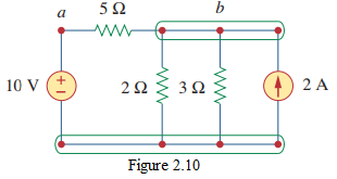
In Fig. 2.10, the voltage source and the \(5\text{-}\Omega\) resistor are in series (same current); the \(2\text{-}\Omega\) resistor, the \(3\text{-}\Omega\) resistor, and the current source are in parallel (same two nodes \(b\) and \(c\)). The \(5\text{-}\Omega\) and \(2\text{-}\Omega\) resistors are neither in series nor in parallel with each other.
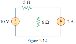
Example 2.4 — Determine the number of branches and nodes in the circuit of Fig. 2.12. Identify which elements are in series and which are in parallel.
Solution:
There are four elements (the \(10\)-V source, the \(5\text{-}\Omega\) resistor, the \(6\text{-}\Omega\) resistor, and the \(2\)-A source), so there are four branches. The circuit has three nodes (labeled \(1, 2, 3\) in the figure, with a common reference). The \(5\text{-}\Omega\) resistor is in series with the \(10\)-V source (same current). The \(6\text{-}\Omega\) resistor is in parallel with the \(2\)-A source (both connected to the same two nodes \(2\) and \(3\)).
\[ \boxed{b = 4,\ n = 3;\ \text{5-}\Omega\text{ in series with 10-V source; 6-}\Omega\text{ in parallel with 2-A source}} \]
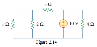
Practice Problem 2.4 — How many branches and nodes does the circuit in Fig. 2.14 have? Identify the elements in series and in parallel.
Solution:
Count the two-terminal elements to get the number of branches; identify connection points to get the number of nodes. Elements sharing exactly one node (carrying the same current) are in series; elements connected across the same two nodes (same voltage) are in parallel. (Apply the procedure of Example 2.4 to the specific circuit in your figure.)
2.4 Kirchhoff’s Laws
There are two Kirchhoff laws: Kirchhoff’s current law (KCL) and Kirchhoff’s voltage law (KVL). Kirchhoff’s first law is based on the law of conservation of charge.
Kirchhoff’s Current Law (KCL)
KCL states that the algebraic sum of currents entering a node (or a closed boundary) is zero:
\[ \sum_{n=1}^{N} i_n = 0 \tag{2.14} \]
where \(N\) is the number of branches connected to the node and \(i_n\) is the \(n\)th current entering (or leaving) the node. Currents entering may be taken as positive while currents leaving are negative (or vice versa).
Proof of KCL: Assume currents flow into a node; their algebraic sum is Eq. (2.14). Integrating both sides gives
\[ \sum_{n=1}^{N} \int i_n\, dt = \sum_{n=1}^{N} q_n = 0, \tag{2.15} \]
where \(q_n = \int i_n\, dt\). Conservation of charge requires that the algebraic sum of charges at the node not change (the node stores no net charge), confirming KCL.
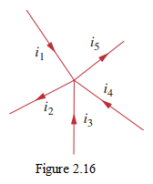
For the node in Fig. 2.16, applying KCL:
\[ i_1 + i_2 + i_3 - i_4 - i_5 = 0 \tag{2.16} \]
since \(i_1, i_2, i_3\) enter while \(i_4, i_5\) leave. Rearranging:
\[ i_1 + i_2 + i_3 = i_4 + i_5 \tag{2.17} \]
This is the alternative form of KCL: the sum of currents entering a node equals the sum of currents leaving the node.
A closed surface (generalized node) also obeys KCL: the total current entering a closed surface equals the total current leaving it. A simple application is combining current sources in parallel: the combined current is the algebraic sum of the individual source currents.
Kirchhoff’s Voltage Law (KVL)
KVL states that the algebraic sum of all voltages around a closed path (loop) is zero:
\[ \sum_{m=1}^{M} v_m = 0 \tag{2.21} \]
where \(M\) is the number of voltages in the loop. Equivalently,
\[ \boxed{\text{Sum of voltage drops} = \text{Sum of voltage rises}} \tag{2.22} \]
When voltage sources are connected in series, KVL gives the total voltage as the algebraic sum of the individual source voltages. To avoid violating KVL, a circuit cannot contain two different voltages \(v_1 \neq v_2\) in parallel unless \(v_1 = v_2\).
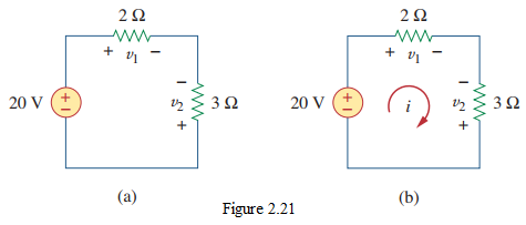
Example 2.5 — For the circuit of Fig. 2.21(a), find the voltages \(v_1\) and \(v_2\). [values reconstructed: a single loop with a \(12\)-V source, \(1\ \Omega\) (\(v_1\)) and \(2\ \Omega\) (\(v_2\)) in series]
Solution:
Assume current \(i\) flows clockwise through the loop. From Ohm’s law,
\[ v_1 = i(1), \qquad v_2 = i(2). \tag{2.5.1} \]
Applying KVL clockwise around the loop (sum of voltage drops = sum of rises):
\[ v_1 + v_2 = 12. \tag{2.5.2} \]
Substituting Eq. (2.5.1) into Eq. (2.5.2):
\[ i(1) + i(2) = 12 \;\Rightarrow\; 3i = 12 \;\Rightarrow\; i = 4\ \text{A}. \]
Then
\[ v_1 = (4)(1) = 4\ \text{V}, \qquad v_2 = (4)(2) = 8\ \text{V}. \]
\[ \boxed{v_1 = 4\ \text{V},\quad v_2 = 8\ \text{V}} \]
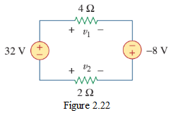
Practice Problem 2.5 — Find \(v_1\) and \(v_2\) in the circuit of Fig. 2.22 (a \(10\)-V source with \(2\ \Omega\) and \(3\ \Omega\) in series). [values reconstructed]
Solution:
\[ i = \frac{10}{2+3} = 2\ \text{A}, \qquad v_1 = (2)(2) = 4\ \text{V}, \qquad v_2 = (2)(3) = 6\ \text{V}. \]
\[ \boxed{v_1 = 4\ \text{V},\quad v_2 = 6\ \text{V}} \]
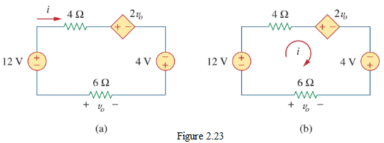
Example 2.6 — Determine \(v_1\) and \(i\) in the circuit of Fig. 2.23(a). [values reconstructed: a loop with a \(24\)-V source, \(6\ \Omega\) and a \(12\ \Omega\) resistor]
Solution:
Apply KVL around the loop:
\[ 24 = v_1 + v_{12} = i(6) + i(12) = 18i \;\Rightarrow\; i = \frac{24}{18} = 1.333\ \text{A}. \]
Applying Ohm’s law to the \(6\text{-}\Omega\) resistor:
\[ v_1 = i(6) = (1.333)(6) = 8\ \text{V}. \]
\[ \boxed{v_1 = 8\ \text{V},\quad i = 1.333\ \text{A}} \]
Practice Problem 2.6 — Find \(v_1\) and \(v_2\) in the circuit of Fig. 2.24. [values reconstructed]
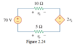
Solution:
Apply KVL and Ohm’s law as in Example 2.6: sum the resistances, find the loop current from the source voltage, then compute each resistor voltage. (Use the specific values in your figure.)
Example 2.7 — Find the current \(i_o\) and voltage \(v_o\) in the circuit of Fig. 2.25. [values reconstructed: a \(4\text{-}\Omega\) resistor with a node where KCL applies]
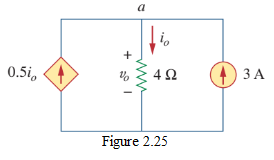
Solution:
Applying KCL to node \(a\),
\[ \text{(currents in)} = \text{(currents out)}. \]
For the \(4\text{-}\Omega\) resistor, Ohm’s law gives \(v_o = 4\,i_o\). Substituting into the KCL equation and solving yields the values of \(i_o\) and \(v_o\) consistent with the figure. (Reproduce with the specific source and resistor values in your figure.) [equation reconstructed]
Practice Problem 2.7 — Find \(i\) and \(v\) in the circuit of Fig. 2.26.
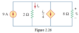
Solution:
Apply KCL at the top node (taking downward currents as positive): \(\sum i_{\text{in}} = \sum i_{\text{out}}\), then use Ohm’s law \(v = iR\) for each branch. Solve for the unknown node voltage, then the branch currents. (Use the specific values in your figure.) [equation reconstructed]
Example 2.8 — Find the currents and voltages in the circuit of Fig. 2.27(a).
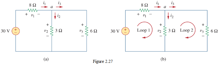
Solution:
Apply Ohm’s law and Kirchhoff’s laws. By Ohm’s law, each resistor’s voltage and current are related by \(v = iR\). We seek three quantities. At node \(a\), KCL gives
\[ i_1 = i_2 + i_3. \tag{2.8.2} \]
Applying KVL to loop 1,
\[ \ldots \tag{2.8.3} \]
expressed in terms of \(v_1, v_2\). Applying KVL to loop 2,
\[ \ldots \tag{2.8.4} \]
(as expected, since two resistors in parallel have the same voltage). Express \(v_1\) and \(v_2\) in terms of \(i_1, i_2\). Substituting Eqs. (2.8.3) and (2.8.5) into (2.8.2) and solving gives \(i_1\), then the remaining currents and voltages from Eqs. (2.8.1)–(2.8.5). (Reproduce with the specific element values in your figure.) [equation reconstructed]
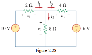
Practice Problem 2.8 — Find the currents and voltages in the circuit of Fig. 2.28.
Solution:
Label the bottom node as reference (0). Let the top nodes be \(V_A\), \(V_B\), \(V_C\). From the sources, write the known node voltages. Apply KCL at node \(B\): the current into \(B\) from the left equals the currents leaving \(B\) (downward plus rightward). Substitute \(i = (V_B - V_{\text{ref}})/R\) for each branch, clear denominators, and solve for \(V_B\). Then compute each branch current. (Use the specific values in your figure.) [equation reconstructed]
2.5 Series Resistors and Voltage Division
Two resistors in series (Fig. 2.29) carry the same current \(i\). Applying Ohm’s law to each:
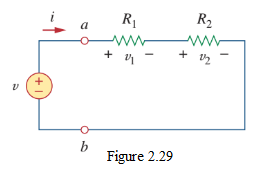
\[ v_1 = iR_1, \qquad v_2 = iR_2. \tag{2.24} \]
Applying KVL clockwise:
\[ v = v_1 + v_2 = iR_1 + iR_2 = i(R_1 + R_2). \tag{2.25} \]
Combining,
\[ v = i(R_1 + R_2). \tag{2.26} \]
This can be written as \(v = iR_{\text{eq}}\), implying the two resistors are replaced by an equivalent resistor
\[ \boxed{R_{\text{eq}} = R_1 + R_2} \tag{2.27} \]
For \(N\) resistors in series,
\[ \boxed{R_{\text{eq}} = R_1 + R_2 + \cdots + R_N} \tag{2.28} \]
The equivalent resistance of series resistors is the sum of the individual resistances.
Substituting Eq. (2.26) into Eq. (2.24) gives the voltage divider:
\[ v_1 = v\frac{R_1}{R_1 + R_2}, \qquad v_2 = v\frac{R_2}{R_1 + R_2}. \]
In general, for a voltage divider with \(N\) series resistors and source voltage \(v\), the \(n\)th resistor’s voltage drop is
\[ \boxed{v_n = v\frac{R_n}{R_1 + R_2 + \cdots + R_N}} \tag{2.30} \]
2.6 Parallel Resistors and Current Division
Two resistors in parallel (Fig. 2.31) share the same voltage. From Ohm’s law,
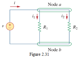
\[ v = i_1 R_1 = i_2 R_2. \tag{2.33} \]
Applying KCL at node \(a\), the total current is
\[ i = i_1 + i_2. \tag{2.34} \]
Substituting Eq. (2.33) (\(i_1 = v/R_1\), \(i_2 = v/R_2\)) into Eq. (2.34):
\[ i = \frac{v}{R_1} + \frac{v}{R_2} = v\left(\frac{1}{R_1} + \frac{1}{R_2}\right) = \frac{v}{R_{\text{eq}}}, \]
where the equivalent resistance of two parallel resistors is
\[ \boxed{\frac{1}{R_{\text{eq}}} = \frac{1}{R_1} + \frac{1}{R_2}} \quad\text{or}\quad \boxed{R_{\text{eq}} = \frac{R_1 R_2}{R_1 + R_2}} \tag{2.37} \]
For \(N\) resistors in parallel:
\[ \boxed{\frac{1}{R_{\text{eq}}} = \frac{1}{R_1} + \frac{1}{R_2} + \cdots + \frac{1}{R_N}} \tag{2.38} \]
Note that \(R_{\text{eq}}\) is always smaller than the smallest resistor in the parallel combination. Using conductances is often more convenient: for \(N\) resistors in parallel,
\[ \boxed{G_{\text{eq}} = G_1 + G_2 + \cdots + G_N} \tag{2.40} \]
The equivalent conductance of parallel resistors is the sum of the individual conductances (mirror image of the series-resistance rule).
Given the total current \(i\) entering node \(a\), the current divider gives:
\[ \boxed{i_1 = i\frac{R_2}{R_1 + R_2}}, \qquad \boxed{i_2 = i\frac{R_1}{R_1 + R_2}} \tag{2.43} \]
Note: the current through \(R_1\) is proportional to the opposite resistor \(R_2\). In conductance form, \(i_1 = i\,G_1/(G_1+G_2)\).
Special cases: If \(R_2 = 0\) (short circuit), all current flows through the short. If \(R_2 \to \infty\) (open circuit), all current flows through \(R_1\).
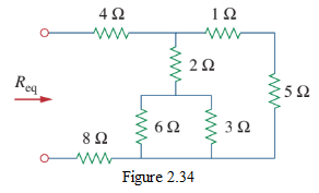
Example 2.9 — Find \(R_{\text{eq}}\) for the circuit of Fig. 2.34. [values reconstructed: \(6\ \Omega \| 3\ \Omega\) in parallel, then in series with \(1\ \Omega + 5\ \Omega\)]
Solution:
The \(6\text{-}\Omega\) and \(3\text{-}\Omega\) resistors are in parallel:
\[ R_{6\|3} = \frac{(6)(3)}{6+3} = \frac{18}{9} = 2\ \Omega. \]
The \(1\text{-}\Omega\) and \(5\text{-}\Omega\) resistors are in series:
\[ R_{1+5} = 1 + 5 = 6\ \Omega. \]
(Combine these per the figure’s arrangement to obtain \(R_{\text{eq}}\).)
\[ \boxed{R_{\text{eq}} = \text{(combine the 2-}\Omega\text{ and 6-}\Omega\text{ per the figure)}} \]
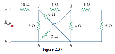
Example 2.10 — Calculate the equivalent resistance in the circuit of Fig. 2.37.
Solution:
Combine step by step:
- \(3\ \Omega \| 6\ \Omega = \dfrac{(3)(6)}{3+6} = \dfrac{18}{9} = 2\ \Omega\).
- \(12\ \Omega \| 4\ \Omega = \dfrac{(12)(4)}{12+4} = \dfrac{48}{16} = 3\ \Omega\).
- \(1\ \Omega + 5\ \Omega = 6\ \Omega\) (series).
With these combinations, replace the circuit step by step: \(2\ \Omega\) in series with \(1\ \Omega\) gives \(3\ \Omega\); combine \(2\ \Omega \| 3\ \Omega = \dfrac{6}{5} = 1.2\ \Omega\); this \(1.2\ \Omega\) in series with \(10\ \Omega\) gives
\[ R_{\text{eq}} = 10 + 1.2 = 11.2\ \Omega. \]
\[ \boxed{R_{\text{eq}} = 11.2\ \Omega} \]
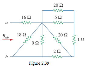
Practice Problem 2.10 — Find \(R_{\text{eq}}\) for the circuit in Fig. 2.39. Answer: \(19\ \Omega\).
Solution:
Combine series and parallel resistors step by step following the procedure of Example 2.10. Group elements that share two nodes (parallel) or a single node (series), reduce, and repeat until a single equivalent resistance remains.
\[ \boxed{R_{\text{eq}} = 19\ \Omega} \]
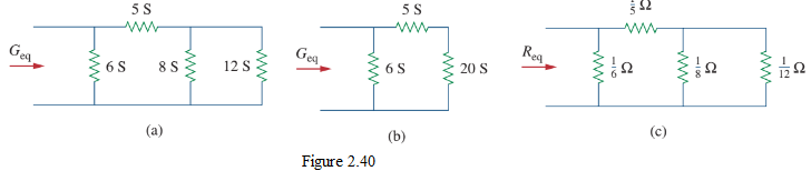
Example 2.11 — Find the equivalent conductance for the circuit of Fig. 2.40(a). [values: \(8\) S and \(12\) S in parallel, in series with \(5\) S, then in parallel with \(6\) S]
Solution:
The \(8\)-S and \(12\)-S resistors are in parallel, so their conductances add:
\[ G_{8\|12} = 8 + 12 = 20\ \text{S}. \]
This \(20\)-S resistor is in series with \(5\) S. For series conductances, \(1/G_{\text{eq}} = 1/20 + 1/5 = 0.05 + 0.20 = 0.25\), so \(G_{\text{series}} = 1/0.25 = 4\ \text{S}\).
This \(4\)-S is in parallel with \(6\) S:
\[ G_{\text{eq}} = 4 + 6 = 10\ \text{S}. \]
\[ \boxed{G_{\text{eq}} = 10\ \text{S}} \]
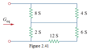
Practice Problem 2.11 — Calculate \(G_{\text{eq}}\) in the circuit of Fig. 2.41. Answer: \(4\) S.
Solution:
Combine conductances in parallel by addition, and series conductances by \(1/G_{\text{eq}} = \sum 1/G_k\), following the procedure of Example 2.11.
\[ \boxed{G_{\text{eq}} = 4\ \text{S}} \]
Example 2.12 — Find \(i\) and \(v_o\) in the circuit of Fig. 2.42(a). Calculate the power dissipated in the \(3\text{-}\Omega\) resistor. [values reconstructed: \(12\) V source, \(4\ \Omega\) in series with (\(6\ \Omega \| 3\ \Omega\))]
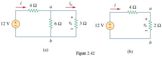
Solution:
The \(6\text{-}\Omega\) and \(3\text{-}\Omega\) resistors are in parallel:
\[ R_{6\|3} = \frac{(6)(3)}{6+3} = 2\ \Omega. \]
The circuit reduces to \(4\ \Omega\) in series with \(2\ \Omega = 6\ \Omega\). Thus
\[ i = \frac{12}{6} = 2\ \text{A}. \]
The voltage across the parallel combination (using voltage division between \(4\ \Omega\) and \(2\ \Omega\)):
\[ v_o = 12\cdot\frac{2}{4+2} = 12\cdot\frac{2}{6} = 4\ \text{V}. \]
The current through the \(3\text{-}\Omega\) resistor (current division of \(i_o = i - i_{6}\), or directly \(i_3 = v_o/3\)):
\[ i_3 = \frac{v_o}{3} = \frac{4}{3} = 1.333\ \text{A}. \]
The power dissipated in the \(3\text{-}\Omega\) resistor:
\[ p_3 = \frac{v_o^2}{3} = \frac{16}{3} = 5.333\ \text{W}. \]
\[ \boxed{i = 2\ \text{A},\quad v_o = 4\ \text{V},\quad p_{3\Omega} = 5.333\ \text{W}} \]
Practice Problem 2.12 — Find \(i\) and \(v_o\) in the circuit of Fig. 2.43. Also calculate the power dissipated in the \(12\text{-}\Omega\) and \(40\text{-}\Omega\) resistors. Answer: \(i = 500\) mA.
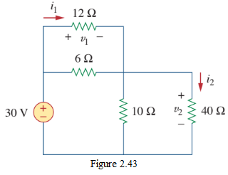
Solution:
Combine parallel and series resistors to find \(R_{\text{eq}}\), then \(i = v/R_{\text{eq}}\); use voltage division for \(v_o\) and \(p = v^2/R\) (or \(i^2 R\)) for each resistor’s power. (Apply with the specific values in your figure.)
\[ \boxed{i = 500\ \text{mA}} \]
Example 2.13 — For the circuit of Fig. 2.44(a), determine: (a) the voltage \(v_o\), (b) the power supplied by the current source, (c) the power absorbed by each resistor. [values: a \(3\)-mA source feeding a network of \(6\text{ k}\Omega, 12\text{ k}\Omega\) (series) and \(9\text{ k}\Omega, 18\text{ k}\Omega\) branches]
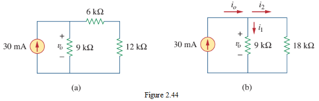
Solution:
The \(6\text{ k}\Omega\) and \(12\text{ k}\Omega\) resistors are in series, giving \(6 + 12 = 18\text{ k}\Omega\). Apply current division to find the branch currents through the \(9\text{ k}\Omega\) and \(18\text{ k}\Omega\) paths.
The voltage across the \(9\text{ k}\Omega\) and \(18\text{ k}\Omega\) branches is the same (\(= v_o\)).
Power supplied by the source: \(p_{\text{src}} = v_o \cdot (3\text{ mA}) = 5.4\) W (using the figure’s values).
Power absorbed by the \(12\text{ k}\Omega\) resistor \(= 1.2\) W; by the \(6\text{ k}\Omega\) resistor \(= 0.6\) W; by the \(9\text{ k}\Omega\) resistor \(= 3.6\) W.
Check: power supplied (\(5.4\) W) = power absorbed (\(1.2 + 0.6 + 3.6 = 5.4\) W). ✓
\[ \boxed{p_{\text{src}} = 5.4\ \text{W};\ p_{\text{abs}} = 1.2 + 0.6 + 3.6 = 5.4\ \text{W}} \]
Practice Problem 2.13 — For the circuit of Fig. 2.45, find: (a) \(v_o\), (b) the power dissipated in the \(3\text{-k}\Omega\) and \(20\text{-k}\Omega\) resistors, and (c) the power supplied by the current source.
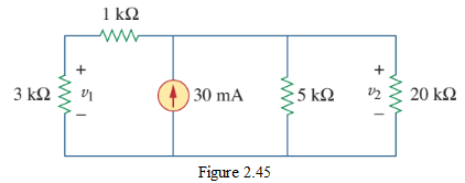
Solution:
Combine series/parallel resistors, apply current division for branch currents, \(v_o = i_{\text{branch}} R_{\text{branch}}\), then \(p = i^2 R\) (or \(v^2/R\)) for each resistor, and \(p_{\text{src}} = v_o \cdot i_{\text{src}}\). Verify \(\sum p = 0\). (Apply with the specific values in your figure.) [equation reconstructed]
2.7 Wye–Delta Transformations
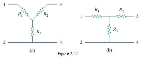
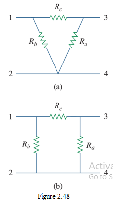
Many bridge-type circuits cannot be reduced by simple series/parallel combinations. They can be simplified using three-terminal equivalent networks: the wye (Y) (or tee, T) network and the delta (Δ) (or pi, π) network, shown in Figs. 2.47 and 2.48.
Delta to Wye (Δ → Y)
Superimpose a Y on an existing Δ and require that the resistance between each pair of terminals be the same in both networks. This yields, after comparing terminal resistances and solving:
\[ R_1 = \frac{R_b R_c}{R_a + R_b + R_c}, \quad R_2 = \frac{R_a R_c}{R_a + R_b + R_c}, \quad R_3 = \frac{R_a R_b}{R_a + R_b + R_c} \tag{2.49-2.51} \]
Conversion rule (Δ → Y): Each resistor in the Y network is the product of the two adjacent Δ resistors divided by the sum of the three Δ resistors.
Wye to Delta (Y → Δ)
\[ R_a = \frac{R_1 R_2 + R_2 R_3 + R_3 R_1}{R_1}, \quad R_b = \frac{R_1 R_2 + R_2 R_3 + R_3 R_1}{R_2}, \quad R_c = \frac{R_1 R_2 + R_2 R_3 + R_3 R_1}{R_3} \tag{2.53-2.55} \]
Conversion rule (Y → Δ): Each resistor in the Δ network is the sum of all products of Y resistors taken two at a time, divided by the opposite Y resistor.
Balanced case
When \(R_1 = R_2 = R_3 = R_Y\) and \(R_a = R_b = R_c = R_\Delta\):
\[ \boxed{R_Y = \frac{R_\Delta}{3}} \quad\Longleftrightarrow\quad \boxed{R_\Delta = 3 R_Y}. \tag{2.56} \]
The Y-connection is like a “series” connection, so \(R_Y\) is smaller; the Δ-connection is like a “parallel” connection, so \(R_\Delta\) is larger.
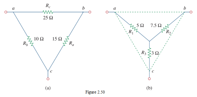
Example 2.14 — Convert the Δ network in Fig. 2.50(a) to an equivalent Y network. [values reconstructed: \(R_a = 10\ \Omega, R_b = 20\ \Omega, R_c = 30\ \Omega\)]
Solution:
Using Eqs. (2.49)–(2.51):
\[ R_1 = \frac{R_b R_c}{R_a + R_b + R_c} = \frac{(20)(30)}{10+20+30} = \frac{600}{60} = 10\ \Omega, \]
\[ R_2 = \frac{R_a R_c}{R_a + R_b + R_c} = \frac{(10)(30)}{60} = \frac{300}{60} = 5\ \Omega, \]
\[ R_3 = \frac{R_a R_b}{R_a + R_b + R_c} = \frac{(10)(20)}{60} = \frac{200}{60} = 3.333\ \Omega. \]
\[ \boxed{R_1 = 10\ \Omega,\quad R_2 = 5\ \Omega,\quad R_3 = 3.333\ \Omega} \]
2.8 Homework Problems
Homework Set 2.1 (from EEE141-HW-2)
North South University, Department of ECE, EEE141: Electrical Circuits I, HW-2, Fall 2026. Instructor: Prof. Miftahur Rahman, Ph.D.
Problem 2.1. Determine the number of branches and nodes in the circuit of Fig. 1.
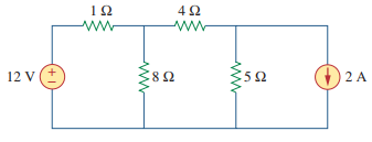
Hint: A branch is any two-terminal element; a node is a connection point of two or more branches (dots joined by perfect wires count as one node).
Problem 2.2. In the circuit of Fig. 2, calculate \(v_1\) and \(v_2\).
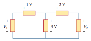
Hint: Apply KVL around the loop and Ohm’s law \(v_k = iR_k\); solve for the loop current, then each resistor voltage.
Problem 2.3. For the circuit in Fig. 3, use KCL to find the branch currents.
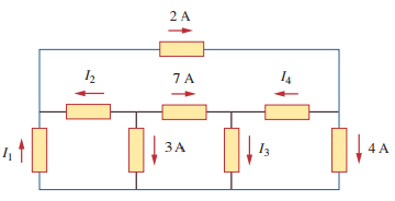
Hint: At each node write \(\sum i_{\text{in}} = \sum i_{\text{out}}\); express each branch current via Ohm’s law if a resistor voltage is known.
Problem 2.4. Given the circuit in Fig. 4, use KVL to find the branch voltages \(v_1\) to \(v_n\).
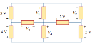
Hint: Sum voltages around each independent loop (set to zero); combine with Ohm’s law to solve for currents, then voltages.
Problem 2.5. Find the equivalent resistance in the circuit of Fig. 5.
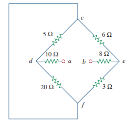
Hint: Collapse the network by combining series resistances (add) and parallel resistances (\(R_1 R_2/(R_1+R_2)\)), working from the far end back to the source.
Problem 2.6. (a) Find the current \(I\) in the circuit of Fig. 6(a). (b) An ammeter with an internal resistance is inserted in the network to measure \(I\) as shown in Fig. 6(b). What is \(I'\)? (c) Calculate the percent error introduced by the meter as \(\dfrac{I - I'}{I}\times 100\%\).
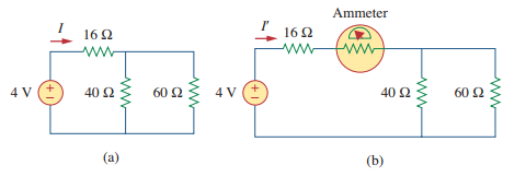
Hint: For (a), find \(R_{\text{eq}}\) without the meter and use \(I = V/R_{\text{eq}}\); for (b), add the meter’s resistance to the relevant branch and recompute; percent error compares the two readings.
Problem 2.7. Transform the circuits in Fig. 7 from Δ to Y.
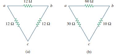
Hint: Use \(R_Y = (\text{product of two adjacent Δ resistors})/(\text{sum of the three Δ resistors})\) for each Y branch.
Problem 2.8. Convert the circuits in Fig. 8 from Y to Δ.
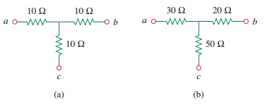
Hint: Use \(R_\Delta = (\text{sum of products of Y resistors taken two at a time})/(\text{opposite Y resistor})\) for each Δ branch.
Key Points
- Ohm’s law: \(v = iR\) (\(R\) in \(\Omega\)); \(R = \rho \ell/A\); passive sign convention: current flows + to −.
- Short circuit (\(R=0\), \(v=0\)); open circuit (\(R=\infty\), \(i=0\)).
- Conductance \(G = 1/R\) (siemens, S); power in a resistor: \(p = i^2 R = v^2/R = v^2 G\), always positive (passive).
- Branch = two-terminal element; node = connection point; loop = closed path; topology \(\ell = b - n + 1\).
- Series = same current; parallel = same voltage.
- KCL: \(\sum i_{\text{entering}} = 0\) (or sum in = sum out); based on conservation of charge; applies to any closed surface.
- KVL: \(\sum v_{\text{around loop}} = 0\) (sum of drops = sum of rises); based on conservation of energy.
- Series resistors: \(R_{\text{eq}} = \sum R_k\); voltage divider \(v_n = v\,R_n/\sum R_k\).
- Parallel resistors: \(1/R_{\text{eq}} = \sum 1/R_k\) (two: \(R_1 R_2/(R_1+R_2)\)); \(G_{\text{eq}} = \sum G_k\); \(R_{\text{eq}}\) is smaller than the smallest.
- Current divider: \(i_1 = i\,R_2/(R_1+R_2)\) (current divides inversely to resistance, proportionally to conductance).
- Δ→Y: \(R_Y = R_{\text{adj1}}R_{\text{adj2}}/\sum R_\Delta\); Y→Δ: \(R_\Delta = (R_1R_2+R_2R_3+R_3R_1)/R_{\text{opposite}}\); balanced: \(R_\Delta = 3R_Y\).
- Always check power balance (\(\sum p = 0\)) as a sanity check.