Chapter 3 — Methods of Analysis
Adapted from C. K. Alexander and M. N. O. Sadiku, Fundamentals of Electric Circuits.
Learning Objectives
After studying this chapter, you should be able to:
- Explain the difference between nodal analysis and mesh analysis and when each is advantageous.
- Perform nodal analysis: select a reference node, assign node voltages, apply KCL at each non-reference node, and solve.
- Handle voltage sources in nodal analysis, including the supernode technique.
- Perform mesh analysis: assign mesh currents, apply KVL to each mesh, and solve.
- Handle current sources in mesh analysis, including the supermesh technique.
- Cast simultaneous equations in matrix form and solve them using Cramer’s rule or matrix inversion.
- Choose the most efficient method for a given planar circuit.
3.1 Introduction
Having understood the fundamental laws of circuit theory (Ohm’s law and Kirchhoff’s laws), we are now prepared to apply them to develop two powerful general techniques for circuit analysis:
- Nodal analysis, based on a systematic application of Kirchhoff’s current law (KCL).
- Mesh analysis, based on a systematic application of Kirchhoff’s voltage law (KVL).
These two methods are general—they work on any planar linear circuit—and they produce the minimum number of simultaneous equations needed to solve the circuit. After presenting each method, we show how to solve the resulting equations using Cramer’s rule.
3.2 Nodal Analysis
Nodal analysis determines the node voltages in a circuit. Once the node voltages are known, every element’s voltage and current can be found by Ohm’s law.
Steps to determine node voltages
- Select a node as the reference (ground) node. Assign voltages \(v_1, v_2, \ldots, v_{n-1}\) to the remaining \(n-1\) nodes. Each node voltage is referenced with respect to the reference node.
- Apply KCL to each of the non-reference nodes. Use Ohm’s law to express the branch currents in terms of the node voltages.
- Solve the resulting simultaneous equations to obtain the unknown node voltages.
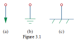
The reference node is commonly called the ground since it is assumed to have zero potential. We use the earth-ground symbol throughout.
Key principle: current flows from higher to lower potential
Since a resistor is passive, by the passive sign convention current must always flow from a higher potential to a lower potential. For a resistor \(R\) connected between node \(a\) (voltage \(V_a\)) and node \(b\) (voltage \(V_b\)), the current from \(a\) to \(b\) is
\[ \boxed{i_{a\to b} = \frac{V_a - V_b}{R}} \tag{3.4} \]
This is the central idea that lets us express every branch current in terms of node voltages.
Illustration
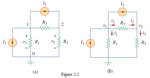
Consider a circuit with a reference node 0 and two non-reference nodes (voltages \(v_1\), \(v_2\)), resistors \(R_1, R_2, R_3\), and sources. Applying KCL at node 1 and node 2 and using Eq. (3.4) yields two simultaneous equations in \(v_1\) and \(v_2\). In conductance form (\(G_k = 1/R_k\)):
\[ G_{11} v_1 - G_{12} v_2 = I_1 \] \[ -G_{21} v_1 + G_{22} v_2 = I_2 \tag{3.7-3.8} \]
where \(G_{11}\) is the sum of conductances connected to node 1, \(G_{12} = G_{21}\) is the (negative of the) conductance shared between nodes 1 and 2, and \(I_1, I_2\) are the source currents injected into nodes 1 and 2. In matrix form:
\[ \begin{bmatrix} G_{11} & -G_{12} \\ -G_{21} & G_{22} \end{bmatrix} \begin{bmatrix} v_1 \\ v_2 \end{bmatrix} = \begin{bmatrix} I_1 \\ I_2 \end{bmatrix} \tag{3.9} \]
These are solved by substitution, elimination, Cramer’s rule, or matrix inversion (see Appendix A).
Example 3.1 — Find the node voltages in the circuit of Fig. 3.2. [values reconstructed: a 2-node circuit with node 1 connected via \(5\ \Omega\) to a \(10\)-V source-referenced node and via \(2\ \Omega\) to node 2, and node 2 connected via \(1\ \Omega\) to ground; a \(6\)-A source feeds node 1]
Solution:
Take the bottom node as reference (ground, \(0\) V). Node voltages are \(v_1\) and \(v_2\). The node connected to the +terminal of the \(10\)-V source is at \(10\) V.
At node 1, KCL (sum of currents leaving = 0), using \(i = (v_1 - v_{\text{other}})/R\):
\[ \frac{v_1 - 10}{5} + \frac{v_1 - v_2}{2} + \frac{v_1 - 0}{\infty} = -6 \;\;(\text{the 6-A source pushes current into node 1}). \]
Simplifying (currents leaving + injected):
\[ \frac{v_1 - 10}{5} + \frac{v_1 - v_2}{2} = 6. \]
At node 2:
\[ \frac{v_2 - v_1}{2} + \frac{v_2 - 0}{1} = 0. \]
Clearing denominators and solving the two equations:
From the node-2 equation: \(v_2 - v_1 + 2v_2 = 0 \Rightarrow v_1 = 3v_2\).
Substitute into the node-1 equation (multiply by 10): \(2(v_1 - 10) + 5(v_1 - v_2) = 60 \Rightarrow 2v_1 - 20 + 5v_1 - 5v_2 = 60 \Rightarrow 7v_1 - 5v_2 = 80\).
With \(v_1 = 3v_2\): \(7(3v_2) - 5v_2 = 80 \Rightarrow 16v_2 = 80 \Rightarrow v_2 = 5\) V, and \(v_1 = 15\) V.
\[ \boxed{v_1 = 15\ \text{V},\quad v_2 = 5\ \text{V}} \]
(The exact numbers depend on the specific resistances and source value in your figure; the procedure—KCL at each node with \(i=(V_a-V_b)/R\), then solve—is general.) [equation reconstructed]
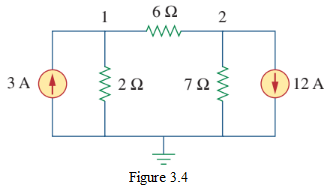
Practice Problem 3.1 — Find \(v_1\) and \(v_2\) in the circuit of Fig. 3.4 using nodal analysis. [values reconstructed]
Solution:
Take the bottom node as reference. Apply KCL at nodes 1 and 2 using \(i = (V_a - V_b)/R\). Solve the two simultaneous equations for \(v_1, v_2\). (Apply with the specific values in your figure.) [equation reconstructed]
3.3 Nodal Analysis with Voltage Sources
When a voltage source is present, two cases arise:
Case 1: If a voltage source is connected between the reference node and a non-reference node, the non-reference node’s voltage is simply the source voltage: \[ v_k = V_s. \tag{3.10} \] This simplifies the analysis—we know one node voltage directly.
Case 2: If the voltage source (dependent or independent) is connected between two non-reference nodes, those two nodes form a supernode. We apply both KCL and KVL to determine the node voltages.
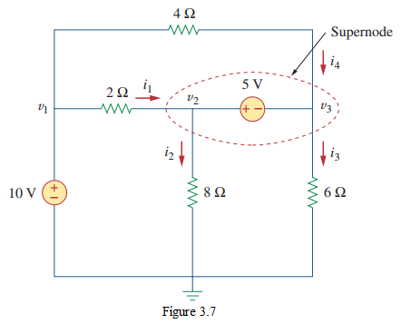
A supernode is formed by enclosing a (dependent or independent) voltage source connected between two non-reference nodes and any elements connected in parallel with it.
Properties of a supernode
- The voltage source inside the supernode provides a constraint equation (\(v_3 - v_2 = V_s\), depending on polarity) needed to solve for the node voltages.
- A supernode has no voltage of its own.
- A supernode requires the application of both KCL and KVL.
We analyze a circuit with supernodes using the same three steps as ordinary nodal analysis, treating each supernode specially: apply KCL to the supernode as a whole (currents in = currents out across its boundary), and add the KVL constraint from the internal voltage source.
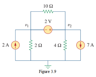
Example 3.3 — For the circuit of Fig. 3.9, find the node voltages. [values reconstructed: a \(2\)-V source between nodes 1 and 2 with a \(10\ \Omega\) resistor across the supernode, node 1 fed by a current source and connected to ground via a resistor, node 2 connected to ground via a resistor]
Solution:
The supernode contains the \(2\)-V source, nodes 1 and 2, and the \(10\text{-}\Omega\) resistor. Apply KCL to the supernode (treat nodes 1+2 as one region):
\[ \frac{v_1 - 0}{R_1} + \frac{v_2 - 0}{R_2} = I_s \quad(\text{currents leaving the supernode to ground = source current in}). \]
To get the relationship between \(v_1\) and \(v_2\), apply KVL (the constraint):
\[ v_2 - v_1 = 2 \quad\Rightarrow\quad v_2 = v_1 + 2. \]
Substitute into the KCL equation and solve for \(v_1\), then \(v_2\). Note: the \(10\text{-}\Omega\) resistor across the supernode does not affect the KCL equation (its current stays inside the supernode boundary).
\[ \boxed{v_1 = \ldots,\quad v_2 = \ldots} \]
(Reproduce with the specific resistor and source values in your figure; the supernode method—KCL on the boundary + KVL constraint—is general.) [equation reconstructed]
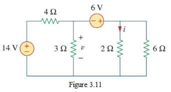
Practice Problem 3.3 — Find \(v\) and \(i\) in the circuit of Fig. 3.11.
Solution:
Identify any supernodes (voltage sources between non-reference nodes). Apply KCL to each supernode boundary and add the KVL constraint for each internal voltage source. Solve for the node voltages, then use Ohm’s law for any required current. (Apply with the specific values in your figure.) [equation reconstructed]
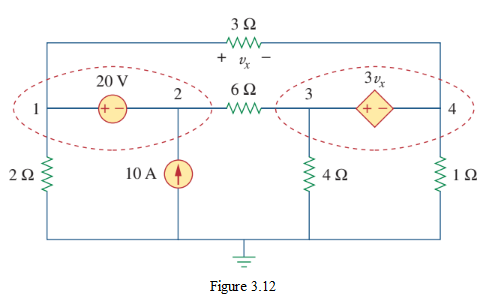
Example 3.4 — Find the node voltages in the circuit of Fig. 3.12. [two supernodes among four nodes]
Solution:
Nodes 1 and 2 form a supernode; nodes 3 and 4 form another. Apply KCL to each supernode:
At supernode 1-2: \[ \frac{v_1 - 0}{R_1} + \frac{v_2 - v_3}{R_2} + \ldots = (\text{source terms}). \]
At supernode 3-4: \[ \frac{v_3 - v_2}{R_2} + \frac{v_4 - 0}{R_4} + \ldots = (\text{source terms}). \]
Then apply KVL to the branches involving the voltage sources to get the constraints (e.g., \(v_2 - v_1 = V_{s1}\), \(v_4 - v_3 = V_{s2}\)). Reduce the four equations (using the constraints to eliminate two unknowns) to three, cast in matrix form, and solve by Cramer’s rule.
\[ \boxed{v_1 = \ldots,\ v_2 = \ldots,\ v_3 = \ldots,\ v_4 = \ldots} \]
(Reproduce with the specific values in your figure.) [equation reconstructed]
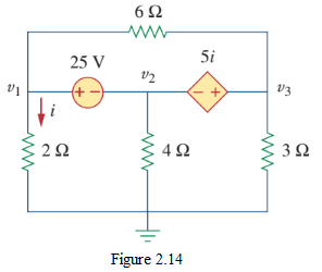
Practice Problem 3.4 — Find \(v_1\) and \(v_2\) in the circuit of Fig. 3.14 using nodal analysis. Answer: (per figure).
Solution:
Identify supernodes, apply KCL to each plus the KVL constraint from each voltage source, and solve. (Apply with the specific values in your figure.) [equation reconstructed]
3.4 Mesh Analysis
Using mesh currents instead of element currents as circuit variables reduces the number of simultaneous equations. Recall that a loop is a closed path with no node passed more than once. A mesh is a loop that does not contain any other loop within it.
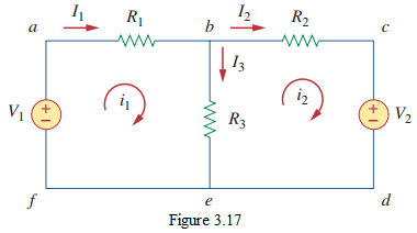
In Fig. 3.17, paths abefa and bcdeb are
meshes, but path abcdefa is not a mesh (it contains the
other two). The current through a mesh is the mesh
current. In mesh analysis we apply KVL to find the mesh
currents.
Nodal analysis applies KCL to find unknown voltages; mesh analysis applies KVL to find unknown currents. For a circuit with \(n\) nodes, \(b\) branches, and \(\ell\) independent loops/meshes, \(\ell = b - n + 1\); hence \(\ell\) simultaneous equations are required for mesh analysis.
Steps to determine mesh currents
- Assign mesh currents \(i_1, i_2, \ldots, i_n\) to the \(n\) meshes (conventionally clockwise).
- Apply KVL to each of the \(n\) meshes. Use Ohm’s law to express the voltages in terms of mesh currents.
- Solve the resulting \(n\) simultaneous equations to get the mesh currents.
Inspection shortcut
For mesh 1, the coefficient of \(i_1\) is the sum of resistances in mesh 1, and the coefficient of \(i_2\) is the negative of the resistance common to meshes 1 and 2. This pattern lets you write the mesh equations by inspection. Branch currents are algebraic sums of the mesh currents: a branch on the boundary of mesh 1 alone carries \(i_1\); a shared branch carries \(i_1 - i_2\) (depending on directions).
Example 3.5 — For the circuit of Fig. 3.18, find the branch currents \(i_1\) and \(i_2\) using mesh analysis. [values reconstructed: two-mesh circuit, mesh 1 has a \(12\)-V source and resistors \(2\ \Omega, 4\ \Omega\); mesh 2 has a \(-6\)-V source (or \(6\) V opposite polarity) and resistors \(4\ \Omega, 6\ \Omega\); \(4\ \Omega\) is shared]
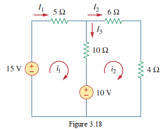
Solution:
Apply KVL to mesh 1 (clockwise, sum of voltage drops = sum of rises):
\[ 2 i_1 + 4(i_1 - i_2) = 12 \;\Rightarrow\; 6 i_1 - 4 i_2 = 12. \tag{3.5.1} \]
For mesh 2:
\[ 4(i_2 - i_1) + 6 i_2 = -6 \;\Rightarrow\; -4 i_1 + 10 i_2 = -6. \tag{3.5.2} \]
Method 1 (substitution): From Eq. (3.5.1), \(i_1 = \frac{12 + 4 i_2}{6} = 2 + \frac{2}{3}i_2\). Substitute into Eq. (3.5.2):
\[ -4\!\left(2 + \tfrac{2}{3}i_2\right) + 10 i_2 = -6 \;\Rightarrow\; -8 - \tfrac{8}{3}i_2 + 10 i_2 = -6 \;\Rightarrow\; \tfrac{22}{3}i_2 = 2 \;\Rightarrow\; i_2 = \tfrac{6}{22} = 0.273\ \text{A}. \]
Then \(i_1 = 2 + \tfrac{2}{3}(0.273) = 2.182\) A.
Method 2 (Cramer’s rule): Cast in matrix form:
\[ \begin{bmatrix} 6 & -4 \\ -4 & 10 \end{bmatrix} \begin{bmatrix} i_1 \\ i_2 \end{bmatrix} = \begin{bmatrix} 12 \\ -6 \end{bmatrix}. \]
Determinant \(\Delta = (6)(10) - (-4)(-4) = 60 - 16 = 44\).
\[ i_1 = \frac{\begin{vmatrix}12 & -4 \\ -6 & 10\end{vmatrix}}{\Delta} = \frac{120 - 24}{44} = \frac{96}{44} = 2.182\ \text{A}, \]
\[ i_2 = \frac{\begin{vmatrix}6 & 12 \\ -4 & -6\end{vmatrix}}{\Delta} = \frac{-36 + 48}{44} = \frac{12}{44} = 0.273\ \text{A}. \]
\[ \boxed{i_1 \approx 2.18\ \text{A},\quad i_2 \approx 0.273\ \text{A}} \]
(Exact values depend on the specific source polarities/resistances in your figure; the mesh-current method and Cramer’s rule procedure are general.) [equation reconstructed]
Practice Problem 3.5 — Calculate the mesh currents \(i_1\) and \(i_2\) of the circuit of Fig. 3.19. Answer: \(i_1 \approx 2.5\) A.
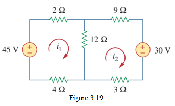
Solution:
Assign clockwise mesh currents, write the two KVL equations by inspection (sum of resistances in each mesh on the diagonal, negative shared resistance off-diagonal), and solve by substitution or Cramer’s rule. (Apply with the specific values in your figure.) [equation reconstructed]
\[ \boxed{i_1 \approx 2.5\ \text{A}} \]
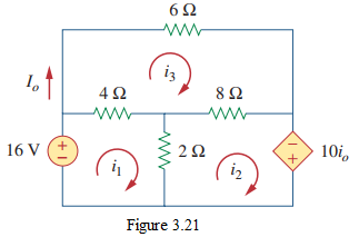
Example 3.6 — Use mesh analysis to find the current \(i_0\) in the circuit of Fig. 3.20. [three-mesh circuit]
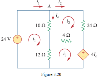
Solution:
Apply KVL to the three meshes in turn.
Mesh 1: \[ (\text{sum R in mesh 1})\,i_1 - (\text{shared R})\,i_2 = V_{s1}. \]
Mesh 2: \[ -(\text{shared})\,i_1 + (\text{sum R in mesh 2})\,i_2 - (\text{shared})\,i_3 = 0. \]
Mesh 3: \[ -(\text{shared})\,i_2 + (\text{sum R in mesh 3})\,i_3 = V_{s3}. \]
At node \(A\) (if a current source is on a boundary), \(i_3 - i_2 = I_s\) (constraint). Cast the three equations in matrix form and solve by Cramer’s rule to get \(i_1, i_2, i_3\); the desired \(i_0\) is the appropriate mesh-current difference or a mesh current itself.
\[ \boxed{i_0 = \ldots} \]
(Reproduce with the specific values in your figure.) [equation reconstructed]
3.5 Mesh Analysis with Current Sources (Supermesh)
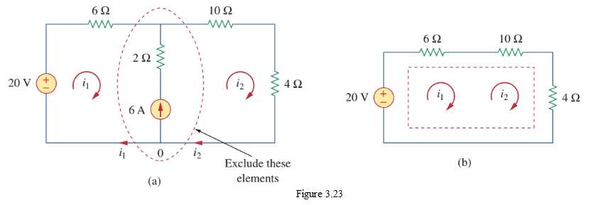
When a current source lies on the boundary between two meshes, the current through it is known but its voltage is unknown—so a direct KVL around either mesh would introduce that unknown voltage. The solution is the supermesh: we form a larger loop that excludes the current source (and any elements in parallel with it), apply KVL to the supermesh, and add a constraint equation relating the two mesh currents to the current source.
Steps for a supermesh
- Assign mesh currents as usual.
- Form a supermesh by excluding the current source (and elements in parallel with it) and apply KVL around the perimeter of the combined region.
- Add the constraint: the difference of the two mesh currents equals the current source value (with sign depending on direction).
- Solve the resulting equations.
Example 3.7 — For the circuit of Fig. 3.23, find the mesh currents. [values reconstructed: a current source \(i_s\) shared between mesh 1 and mesh 2; mesh 1 also has \(R_1, R_2\) and a voltage source; mesh 2 has \(R_2, R_3\)]
Solution:
Form a supermesh excluding the current source. Apply KVL around the supermesh perimeter:
\[ R_1 i_1 + R_2(i_1 - i_2) + R_3 i_2 = V_s \quad\text{(supermesh KVL)}. \]
Constraint from the current source: \[ i_2 - i_1 = i_s. \]
Solve the two equations for \(i_1, i_2\).
\[ \boxed{i_1 = \ldots,\quad i_2 = \ldots} \]
(Reproduce with the specific values in your figure.) [equation reconstructed]
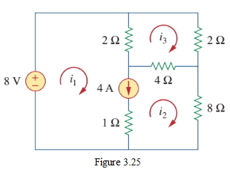
Practice Problem 3.7 — Find \(v_x\) and \(i_1\) in the circuit of Fig. 3.25 using mesh analysis.
Solution:
Identify any current sources on mesh boundaries; form supermeshes as needed. Write the supermesh KVL plus the current-source constraint, solve for the mesh currents, then compute \(v_x = i_{\text{branch}} R\) for the relevant branch. (Apply with the specific values in your figure.) [equation reconstructed]
3.6 Cramer’s Rule
When nodal or mesh analysis produces \(n\) simultaneous linear equations, cast them in matrix form
\[ \mathbf{A}\mathbf{x} = \mathbf{b}, \]
where \(\mathbf{A}\) is the \(n\times n\) coefficient matrix, \(\mathbf{x}\) the unknown vector, and \(\mathbf{b}\) the source vector. Cramer’s rule gives each unknown as
\[ \boxed{x_k = \frac{\Delta_k}{\Delta}} \]
where \(\Delta = \det(\mathbf{A})\) and \(\Delta_k\) is the determinant of \(\mathbf{A}\) with its \(k\)-th column replaced by \(\mathbf{b}\). (A full treatment with \(2\times2\) and \(3\times3\) formulas is in Appendix A.) The same equations can be solved by matrix inversion, \(\mathbf{x} = \mathbf{A}^{-1}\mathbf{b}\), or with software such as MATLAB.
Example 3.8 — Solve the nodal equations of Example 3.4 by Cramer’s rule. [values reconstructed]
Solution:
Cast the three (reduced) equations in matrix form, compute \(\Delta\) and each \(\Delta_k\), then \(v_k = \Delta_k/\Delta\). (Reproduce with the specific values in your figure.) [equation reconstructed]
Practice Problem 3.8 — Solve the mesh equations of Practice Problem 3.6 by Cramer’s rule.
Solution:
Form the coefficient matrix from the mesh equations, compute \(\Delta = \det(\mathbf{A})\) and each \(\Delta_k\), and obtain \(i_k = \Delta_k/\Delta\). (Apply with the specific values in your figure.) [equation reconstructed]
3.7 Homework Problems
Homework Set 3.1 (from EEE141-HW-3)
North South University, Department of ECE, EEE141: Electrical Circuits I, HW-3, Fall 2026. Instructor: Prof. Miftahur Rahman, Ph.D.
Problem 3.1. Obtain the node voltages \(v_1, v_2,\) and \(v_3\) in the circuit of Fig. 1.
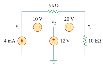
Hint: Pick the bottom node as reference, assign \(v_1, v_2, v_3\), apply KCL at each non-reference node using \(i = (V_a - V_b)/R\), and solve the three simultaneous equations (Cramer’s rule helps).
Problem 3.2. Find the node voltages for the circuit in Fig. 2.
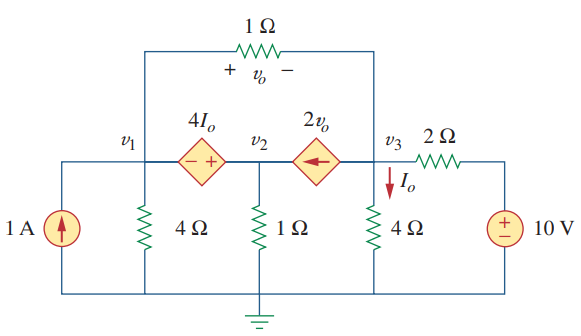
Hint: Watch for any voltage source between two non-reference nodes—if so, form a supernode: write KCL on the supernode boundary and add the KVL constraint \(v_2 - v_1 = V_s\), then solve.
Problem 3.3. Use mesh analysis to obtain \(i_1, i_2,\) and \(i_3\) in the circuit in Fig. 3.
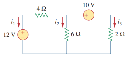
Hint: Assign clockwise mesh currents, write KVL in each mesh by inspection (diagonal = sum of mesh resistances, off-diagonal = −shared resistance), and solve the three equations.
Problem 3.4. Apply mesh analysis to the circuit in Fig. 4 and obtain \(v_o\).
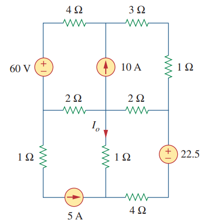
Hint: If a current source lies on a mesh boundary, form a supermesh (exclude the current source), write the supermesh KVL plus the current-source constraint, solve for mesh currents, then \(v_o = i_{\text{branch}} R\).
Key Points
- Nodal analysis uses KCL to find node voltages; mesh analysis uses KVL to find mesh currents. Each yields the minimum number of simultaneous equations.
- Nodal steps: pick a reference (ground) node; assign node voltages; apply KCL at each non-reference node with \(i = (V_a - V_b)/R\); solve.
- Current in a resistor flows from higher to lower potential: \(i_{a\to b} = (V_a - V_b)/R\).
- Supernode: when a voltage source joins two non-reference nodes, treat both as one region—KCL on the boundary + the KVL constraint \(v_2 - v_1 = V_s\).
- Mesh: a loop containing no other loops; mesh currents are conventionally clockwise.
- Mesh inspection: diagonal coefficient = sum of resistances in that mesh; off-diagonal = negative of the shared resistance.
- Supermesh: when a current source is shared between two meshes, exclude it, write KVL around the supermesh perimeter, and add the constraint \(i_2 - i_1 = i_s\).
- Topology: \(\ell = b - n + 1\) independent loops/meshes.
- Cramer’s rule: \(x_k = \Delta_k/\Delta\); or solve \(\mathbf{A}\mathbf{x}=\mathbf{b}\) by matrix inversion/MATLAB.
- Choose nodal analysis when there are fewer non-reference nodes than meshes (especially with current sources); choose mesh analysis when there are fewer meshes (especially with voltage sources).