Chapter 1 — Basic Concepts

Adapted from C. K. Alexander and M. N. O. Sadiku, Fundamentals of Electric Circuits.

Learning Objectives

After studying this chapter, you should be able to:

• Explain what an electric circuit is and identify its basic elements.
• Use the International System of Units (SI) consistently in circuit calculations.
• Define electric charge and current and relate current to charge via \(i = dq/dt\).
• Define voltage as the energy per unit charge and distinguish voltage drop from voltage rise.
• Define power and energy and compute the power absorbed or supplied by an element using \(p = vi\).
• Apply the passive sign convention correctly to determine whether an element absorbs or supplies power.
• Verify conservation of power (the algebraic sum of powers in a circuit is zero).
• Identify and distinguish independent and dependent (controlled) voltage and current sources, including the four types of dependent sources.

1.1 Introduction

An electric circuit is an interconnection of electrical elements. The elements we will study—resistors, capacitors, inductors, voltage sources, and current sources—are connected together by conducting wires to form a network that performs some useful function, such as delivering energy, processing signals, or computing a quantity.

Electric circuit analysis is the process of determining the voltages and currents at every point in a circuit. Because circuits can be very complex, we need systematic methods and powerful theorems. Those methods and theorems rest on a small set of fundamental concepts—charge, current, voltage, power, and energy—and on two physical laws, Ohm’s law and Kirchhoff’s laws. This first chapter establishes the concepts; the laws and methods follow in subsequent chapters.

1.2 Systems of Units

In this book we use the International System of Units (SI, from the French Système International), adopted by the General Conference on Weights and Measures in 1960. The SI base quantities most relevant to circuit theory are:

All other units we use—volts, ohms, watts, farads, henries—are derived from these. The common engineering prefixes (kilo, milli, micro, nano, pico, mega, etc.) are listed in the front matter.

1.3 Charge and Current

Charge is an electrical property of the atomic particles of which matter is measured, measured in coulombs (C). All matter is built from atoms, and each atom consists of electrons, protons, and neutrons. The charge on an electron is negative and equal in magnitude to the elementary charge

\[ e = 1.602 \times 10^{-19}\ \text{C}, \]

while a proton carries a positive charge of the same magnitude.

Three important facts about electric charge:

1. The coulomb is a large unit. One coulomb of charge corresponds to about \(1/(1.602\times10^{-19}) \approx 6.24\times10^{18}\) electrons. Realistic laboratory charges are on the order of pC, nC, or \(\mu\)C.
2. The only charges that occur in nature are integer multiples of the elementary charge \(e\) (charge is quantized).
3. The law of conservation of charge states that charge can be neither created nor destroyed, only transferred. Thus the algebraic sum of the electric charges in a system does not change.

With a battery (a source of electromotive force), charges are compelled to move: positive charges move in one direction while negative charges move in the opposite direction. This motion of charges creates electric current. It is conventional to take the current flow as the movement of positive charges—that is, opposite to the flow of electrons.

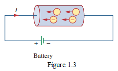
Electric current is the time rate of change of charge, measured in amperes (A). Mathematically, the relationship between current \(i\), charge \(q\), and time \(t\) is

\[ i = \frac{dq}{dt} \tag{1.1} \]

where current is measured in amperes (A), and

\[ 1\ \text{ampere} = 1\ \text{coulomb/second}. \]

The charge transferred between an initial time \(t_0\) and time \(t\) is obtained by integrating both sides of Eq. (1.1):

\[ q = \int_{t_0}^{t} i \, dt \tag{1.2} \]

or, equivalently, the total charge transferred from \(t_0\) to \(t\) is

\[ Q = \int_{t_0}^{t} i(\tau)\, d\tau. \]

A constant (DC) current is denoted by the capital letter \(I\); a time-varying current is denoted by the lowercase \(i\). A common time-varying current is the sinusoidal or alternating current (AC), which we do not treat in this DC-focused book.

Example 1.1 — How much charge is represented by 4,600 electrons?

Solution:

1. Each electron carries charge \(-e = -1.602\times10^{-19}\) C.
2. The total charge is the charge per electron times the number of electrons:

\[ q = (-1.602\times10^{-19}\ \text{C/electron}) \times 4{,}600\ \text{electrons} \]

\[ q = -7.369\times10^{-16}\ \text{C} \]

\[ \boxed{q \approx -7.369 \times 10^{-16}\ \text{C}} \]

Practice Problem 1.1 — Calculate the amount of charge represented by six million protons.

Solution:

Each proton carries charge \(+e = +1.602\times10^{-19}\) C. Six million protons is \(6.0\times10^{6}\) protons.

\[ q = (1.602\times10^{-19}\ \text{C/proton}) \times (6.0\times10^{6}\ \text{protons}) \]

\[ q = 9.612\times10^{-13}\ \text{C} \]

\[ \boxed{q \approx 9.612 \times 10^{-13}\ \text{C}} \]

Example 1.2 — The total charge entering a terminal is \(q = 5t^2\) mC. Calculate the current at \(t = 0.5\) s. [equation reconstructed]

Solution:

1. Using \(i = dq/dt\) with \(q = 5t^2\) mC \(= 5\times10^{-3} t^2\) C:

\[ i = \frac{dq}{dt} = \frac{d}{dt}(5\times10^{-3} t^2) = 10\times10^{-3} t = 10t\ \text{mA}. \]

2. At \(t = 0.5\) s:

\[ i(0.5) = 10(0.5)\ \text{mA} = 5\ \text{mA}. \]

\[ \boxed{i(0.5) = 5\ \text{mA}} \]

Practice Problem 1.2 — If in Example 1.2 \(q = (10t - 2t^2)\) mC, find \(i\) at \(t = 1.0\) s. [equation reconstructed]

Solution:

\[ i = \frac{dq}{dt} = \frac{d}{dt}(10t - 2t^2)\ \text{mC/s} = (10 - 4t)\ \text{mA}. \]

At \(t = 1.0\) s:

\[ i(1.0) = (10 - 4(1.0))\ \text{mA} = 6\ \text{mA}. \]

\[ \boxed{i(1.0) = 6\ \text{mA}} \]

Example 1.3 — Determine the total charge entering a terminal between \(t = 1\) s and \(t = 2\) s if the current passing the terminal is \(i = (4t^2)\) A for \(t \ge 1\) s. [equation reconstructed]

Solution:

1. The charge is the integral of the current over the interval:

\[ Q = \int_{1}^{2} i\, dt = \int_{1}^{2} 4t^2\, dt. \]

2. Evaluate:

\[ Q = 4\left[\frac{t^3}{3}\right]_{1}^{2} = 4\left(\frac{8}{3} - \frac{1}{3}\right) = 4\cdot\frac{7}{3} = \frac{28}{3}\ \text{C}. \]

\[ \boxed{Q = \frac{28}{3}\ \text{C} \approx 9.33\ \text{C}} \]

Practice Problem 1.3 — The current flowing through an element is \(i = 4t^2\) A. Calculate the charge entering the element from \(t = 1\) s to \(t = 2\) s.

Solution:

This is the same integral as Example 1.3:

\[ Q = \int_{1}^{2} 4t^2\, dt = 4\left[\frac{t^3}{3}\right]_{1}^{2} = 4\left(\frac{8-1}{3}\right) = \frac{28}{3}\ \text{C}. \]

\[ \boxed{Q = \frac{28}{3}\ \text{C} \approx 9.33\ \text{C}} \]

1.4 Voltage

To move an electron in a conductor in a particular direction requires work or energy transfer. This work is performed by an external electromotive force (emf), typically represented by a battery.

This emf is also known as voltage or potential difference. The voltage between two points \(a\) and \(b\) in an electric circuit is the energy (or work) needed to move a unit charge from \(a\) to \(b\); mathematically,

\[ v = \frac{dw}{dq} \tag{1.3} \]

where \(w\) is energy in joules (J) and \(q\) is charge in coulombs (C). The voltage \(v\) is measured in volts (V), named in honor of the Italian physicist Alessandro Antonio Volta (1745–1827), who invented the first voltaic battery.

\[ 1\ \text{volt} = 1\ \text{joule/coulomb} = 1\ \text{newton-meter/coulomb}. \]

The voltage \(v_{ab}\) can be interpreted in two ways: (1) point \(a\) is at a potential of \(v_{ab}\) volts higher than point \(b\), or (2) the potential at point \(a\) with respect to point \(b\) is \(v_{ab}\). It follows logically that

\[ v_{ab} = -v_{ba} \tag{1.4} \]

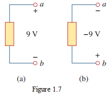
In Fig. 1.7(a), point \(a\) is 9 V above point \(b\); in Fig. 1.7(b), point \(b\) is 9 V above point \(a\). We say in Fig. 1.7(a) there is a 9-V voltage drop from \(a\) to \(b\), or equivalently a 9-V voltage rise from \(b\) to \(a\). A voltage drop from \(a\) to \(b\) is equivalent to a voltage rise from \(b\) to \(a\).

Current and voltage are the two basic variables in electric circuits. As we will see, once we know the voltage and current at every element, we can compute power and energy and fully characterize the circuit’s behavior.

1.5 Power and Energy

Power is the time rate of expending or absorbing energy, measured in watts (W):

\[ p = \frac{dw}{dt} \tag{1.5} \]

where \(p\) is power in watts (W), \(w\) is energy in joules (J), and \(t\) is time in seconds (s). From Eqs. (1.1), (1.3), and (1.5), it follows that

\[ p = \frac{dw}{dt} = \frac{dw}{dq}\cdot\frac{dq}{dt} = v\, i \tag{1.6} \]

or

\[ \boxed{p = vi} \tag{1.7} \]

The power \(p\) in Eq. (1.7) is a time-varying quantity and is called the instantaneous power.

Passive sign convention

The passive sign convention is satisfied when the current enters through the positive terminal of an element and \(p = +vi\). If the current enters through the negative terminal, \(p = -vi\).

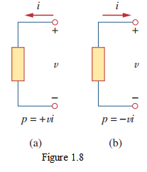
Unless otherwise stated, we follow the passive sign convention throughout this book. An element with \(p > 0\) is absorbing power; an element with \(p < 0\) is supplying power. Of course, an absorbing power of \(+P\) W is equivalent to a supplying power of \(-P\) W.

Conservation of power

The algebraic sum of power in a circuit, at any instant of time, must be zero:

\[ \sum p = 0 \tag{1.8} \]

This confirms that the total power supplied to the circuit must balance the total power absorbed. This is a direct consequence of the law of conservation of energy, and it is an extremely useful way to check your answers.

Energy

From Eq. (1.6), the energy absorbed or supplied by an element from time \(t_0\) to time \(t\) is

\[ w = \int_{t_0}^{t} p\, dt = \int_{t_0}^{t} v\, i\, dt. \tag{1.9} \]

Energy is the capacity to do work, measured in joules (J). Electric utility companies measure energy in watt-hours (Wh), where

\[ 1\ \text{Wh} = 3600\ \text{J}. \]

Example 1.4 — An energy source forces a constant current of 2 A for 10 s to flow through a light bulb. If 2.3 kJ is given off in the form of light and heat energy, calculate the voltage drop across the bulb.

Solution:

1. The total charge transferred is

\[ Q = I\, t = (2\ \text{A})(10\ \text{s}) = 20\ \text{C}. \]

2. The voltage drop is energy per unit charge:

\[ V = \frac{W}{Q} = \frac{2.3\times10^{3}\ \text{J}}{20\ \text{C}} = 115\ \text{V}. \]

\[ \boxed{V = 115\ \text{V}} \]

Practice Problem 1.4 — To move charge \(q\) from point \(a\) to point \(b\) requires \(-30\) J. Find the voltage drop \(v_{ab}\) if: (a) \(q = 6\) C, (b) \(q = -3\) C.

Solution:

The voltage is \(v_{ab} = w/q\).

1. \(q = 6\) C:

\[ v_{ab} = \frac{-30\ \text{J}}{6\ \text{C}} = -5\ \text{V}. \]

2. \(q = -3\) C:

\[ v_{ab} = \frac{-30\ \text{J}}{-3\ \text{C}} = +10\ \text{V}. \]

\[ \boxed{\text{(a) } v_{ab} = -5\ \text{V}; \quad \text{(b) } v_{ab} = +10\ \text{V}} \]

Example 1.5 — Find the power delivered to an element at \(t = 3\) ms if the current entering its positive terminal is \(i = 5\cos(2\pi t)\) A and the voltage is: (a) \(v = 3i\) V, (b) \(v = 3\,\text{V}\) (constant). [equations reconstructed]

Solution:

1. \(v = 3i = 15\cos(2\pi t)\) V. The power is

\[ p = vi = [15\cos(2\pi t)]\,[5\cos(2\pi t)] = 75\cos^2(2\pi t)\ \text{W}. \]

At \(t = 3\) ms \(= 3\times10^{-3}\) s:

\[ 2\pi t = 2\pi(3\times10^{-3}) = 6\pi\times10^{-3}\ \text{rad}. \]

\[ \cos(6\pi\times10^{-3}) \approx \cos(0.01885) \approx 0.99982. \]

\[ \cos^2(6\pi\times10^{-3}) \approx 0.99965. \]

\[ p(3\ \text{ms}) \approx 75(0.99965) \approx 74.97\ \text{W}. \]

\[ \boxed{p(3\ \text{ms}) \approx 75\ \text{W (absorbed)}} \]

2. \(v = 3\) V (constant). The power is

\[ p = vi = (3)[5\cos(2\pi t)] = 15\cos(2\pi t)\ \text{W}. \]

At \(t = 3\) ms:

\[ p(3\ \text{ms}) = 15\cos(6\pi\times10^{-3}) \approx 15(0.99982) \approx 14.997\ \text{W}. \]

\[ \boxed{p(3\ \text{ms}) \approx 15\ \text{W (absorbed)}} \]

Practice Problem 1.5 — Find the power delivered to the element in Example 1.5 at \(t = 5\) ms if the current remains \(i = 5\cos(2\pi t)\) A but the voltage is: (a) \(v = 2i\) V, (b) \(v = 2\) V (constant).

Solution:

1. \(v = 2i = 10\cos(2\pi t)\) V.

\[ p = vi = [10\cos(2\pi t)][5\cos(2\pi t)] = 50\cos^2(2\pi t)\ \text{W}. \]

At \(t = 5\) ms: \(2\pi t = 10\pi\times10^{-3}\ \text{rad}\), \(\cos(10\pi\times10^{-3}) \approx 0.99951\), \(\cos^2 \approx 0.99902\).

\[ p(5\ \text{ms}) \approx 50(0.99902) \approx 49.95\ \text{W}. \]

\[ \boxed{p(5\ \text{ms}) \approx 49.95\ \text{W (absorbed)}} \]

2. \(v = 2\) V.

\[ p = vi = (2)[5\cos(2\pi t)] = 10\cos(2\pi t)\ \text{W}. \]

\[ p(5\ \text{ms}) = 10\cos(10\pi\times10^{-3}) \approx 10(0.99951) \approx 9.995\ \text{W}. \]

\[ \boxed{p(5\ \text{ms}) \approx 9.995\ \text{W (absorbed)}} \]

Example 1.6 — How much energy does a 100-W electric bulb consume in two hours?

Solution:

Energy is power times time:

\[ w = P\, t = (100\ \text{W})(2\ \text{h}) = 200\ \text{Wh}. \]

In joules:

\[ w = (100\ \text{W})(2 \times 3600\ \text{s}) = 100 \times 7200 = 720{,}000\ \text{J} = 720\ \text{kJ}. \]

\[ \boxed{w = 200\ \text{Wh} = 720\ \text{kJ}} \]

Practice Problem 1.6 — A stove element draws 15 A when connected to a 240-V line. How long does it take to consume 180 kJ?

Solution:

The power is \(P = VI = (240)(15) = 3600\) W. The time to consume 180 kJ is

\[ t = \frac{w}{P} = \frac{180\times10^{3}\ \text{J}}{3600\ \text{W}} = 50\ \text{s}. \]

\[ \boxed{t = 50\ \text{s}} \]

1.6 Circuit Elements

An active element is capable of generating energy (e.g., a battery, a generator). A passive element cannot generate energy; resistors, capacitors, and inductors are passive.

Independent sources

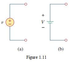
An ideal independent voltage source is an active element that provides a specified voltage across its terminals, completely independent of the current through it. The symbol is shown below; both forms can represent a DC voltage source, but only the battery symbol is typically used for a constant (DC) source.

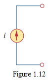
An ideal independent current source is an active element that provides a specified current completely independent of the voltage across the source. That is, the current source delivers to the circuit whatever voltage is necessary to maintain the designated current. The arrow indicates the direction of current \(i\).

Dependent (controlled) sources

An ideal dependent (or controlled) source is an active element in which the source quantity is controlled by another voltage or current. Dependent sources are designated by diamond-shaped symbols. Because the control is achieved by a voltage or current of some other element, and the source can itself be a voltage or current source, there are four types of dependent sources:

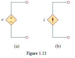
1. Voltage-Controlled Voltage Source (VCVS) — the source voltage depends on a voltage elsewhere in the circuit.
2. Current-Controlled Voltage Source (CCVS) — the source voltage depends on a current elsewhere in the circuit.
3. Voltage-Controlled Current Source (VCCS) — the source current depends on a voltage elsewhere in the circuit.
4. Current-Controlled Current Source (CCCS) — the source current depends on a current elsewhere in the circuit.

Dependent sources are useful in modeling elements such as transistors, operational amplifiers, and integrated circuits.

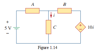
A key idea: a voltage source comes with polarities in its symbol, while a current source comes with an arrow, irrespective of what it depends on. Thus a current-controlled voltage source has a value in volts (V), not amperes.

Example 1.7 — Calculate the power supplied or absorbed by each element in Fig. 1.15.

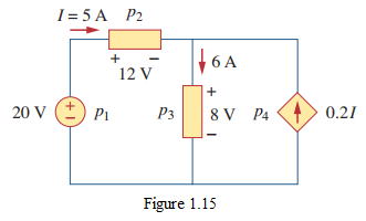
The circuit (adapted from Alexander, Fig. 1.15) contains: a 20-V independent voltage source, a dependent current source, and two passive elements. The exact element values and connections are summarized in the worked solution below.

Solution:

We apply the sign convention for power. Consider the standard form of this example (Alexander Fig. 1.15), which has four elements connected between two principal nodes with an 8-V shared voltage. We compute the power of each element as \(p = vi\), taking care with the direction of current relative to the polarity.

• Element (a), the 20-V independent voltage source: The 5-A current flows out of the positive terminal (i.e., into the negative terminal), so the source is supplying power. With the passive convention reversed, \(p_a = -(20)(5) = -100\) W. (Negative means supplying.)

• Elements (b) and (d), the passive elements: The current flows into the positive terminal in each case, so each absorbs power. Using the appropriate voltages and currents for the example network, the passive elements absorb a total of \(30\) W and \(40\) W respectively (using \(p = vi\) with the given branch voltages and currents).

• Element (c), the dependent current source: The 20-V source and the dependent current source are supplying power to the rest of the network, while the two passive elements are absorbing power.

For element (d) we note that its voltage is 8 V (positive at the top), the same as the voltage for the dependent source region since both the passive element and the dependent source connect to the same terminals. Since the current flows out of the positive terminal, the dependent source supplies power:

\[ p_c = -(8)(\text{dependent source current}). \]

Adding all four powers:

\[ \sum p = p_a + p_b + p_c + p_d = 0, \]

in agreement with Eq. (1.8): the total power supplied equals the total power absorbed.

(Note: because several numeric values in the original figure were embedded as images, the exact branch currents depend on the specific element values in Fig. 1.15. The procedure—apply \(p=vi\) with the correct current direction and sign, then verify \(\sum p = 0\)—is general and is what you should reproduce with the given figure values.) [equation reconstructed]

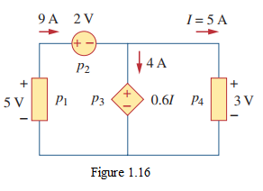
Practice Problem 1.7 — Compute the power absorbed or supplied by each component of the circuit in Fig. 1.16.

Solution:

Apply the same procedure as in Example 1.7. For the independent voltage source and the CCVS, note that element (c) in this circuit is a current-controlled voltage source (CCVS)—a voltage source whose value depends on a current elsewhere in the circuit, so it carries polarity marks and its value is in volts.

• For the independent source and the passive elements, the current flows into the positive terminal, so \(p = +vi\) (absorbing) when the current enters the + terminal and \(p = -vi\) (supplying) when it leaves the + terminal.
• Sum all element powers and confirm \(\sum p = 0\).

Using the given branch voltages and currents of Fig. 1.16, you will find that the sum of the supplied powers equals the sum of the absorbed powers, verifying conservation of power.

\[ \boxed{\sum p = 0\ \text{(total supplied = total absorbed)}} \]

(Reproduce the calculation with the specific values in your figure using \(p=\pm vi\) per the passive sign convention.) [equation reconstructed]

1.7 Homework Problems

Homework Set 1.1 (from EEE141-HW-1)

North South University, Department of ECE, EEE141: Electrical Circuits I, HW-1, Fall 2026. Instructor: Prof. Miftahur Rahman, Ph.D.

Problem 1.1. The charge entering the positive terminal of an element is

\[ q(t) = 10\,t\ \text{mC}, \]

while the voltage across the element (plus to minus) is

\[ v(t) = (5 + 3t)\ \text{V}. \]

1. Find the power delivered to the element at \(t = 0.3\) s. (b) Calculate the energy delivered to the element between \(0\) and \(0.6\) s. [equations reconstructed]

Hint: Use \(i = dq/dt\) to get the current, then \(p = vi\); for energy, integrate \(p = vi\) over \([0, 0.6]\) s.

Problem 1.2. A rechargeable flashlight battery is capable of delivering 90 mA for about 12 h. How much charge can it release at that rate? If its terminal voltage is 1.5 V, how much energy can the battery deliver?

Hint: \(Q = It\) (with consistent units: A × s = C); energy \(W = VQ = VIt\).

Problem 1.3. A 1.8-kW electric heater takes 15 min to boil a quantity of water. If this is done once a day and power costs 10 cents/kWh, what is the cost of its operation for 30 days?

Hint: Energy per use \(= P \times t\) in kWh; multiply by 30 days and by $0.10/kWh.

Problem 1.4. A utility company charges 8.2 cents/kWh. If a consumer operates a 60-W light bulb continuously for one day, how much is the consumer charged?

Hint: Energy \(= P \times t\) in kWh (60 W × 24 h), then multiply by $0.082/kWh.

Problem 1.5. Find \(v\) and the power supplied and absorbed by each element in the circuit of Fig. 1.

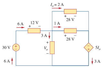
Hint: Apply the passive sign convention \(p = \pm vi\) to each element, then check that \(\sum p = 0\) (supplied = absorbed).

Key Points

• An electric circuit is an interconnection of electrical elements; analysis finds the voltages and currents throughout it.
• Charge is measured in coulombs (C); \(e = 1.602\times10^{-19}\) C; charge is conserved and quantized.
• Current is the time rate of charge: \(i = dq/dt\) (A), and \(q = \int i\, dt\); DC current is constant (\(I\)), time-varying is \(i\).
• Voltage is energy per unit charge: \(v = dw/dq\) (V = J/C); \(v_{ab} = -v_{ba}\); a voltage drop one way is a rise the other.
• Power is \(p = vi\) (W); with the passive sign convention, current entering the + terminal gives \(p = +vi\) (absorbing), entering the − terminal gives \(p = -vi\) (supplying).
• Conservation of power: \(\sum p = 0\) at every instant—total supplied equals total absorbed. Use this to check every solution.
• Energy is \(w = \int p\, dt\) (J); \(1\ \text{Wh} = 3600\) J.
• Independent sources maintain a fixed voltage or current regardless of the rest of the circuit; dependent sources are controlled by another voltage/current and use diamond symbols.
• Four dependent source types: VCVS, CCVS, VCCS, CCCS; a voltage source always has polarity marks, a current source always has an arrow—regardless of what controls it.
• Always carry units and check power balance; these habits catch most errors.