Chapter 14 Oscillations

Learning Objectives:

In this chapter you will basically learn:

\(\bullet\) Simple harmonic motion from other types of periodic motion.

\(\bullet\) For a simple harmonic oscillator, apply the relationship between position x and time t to calculate either if given a value for the other.

\(\bullet\) Relate period T, frequency f, and angular frequency \(\omega\).

\(\bullet\) Identify (displacement) amplitude \(x_m\), phase constant (or phase angle) \(\phi\), and phase \(\phi + \omega t\).

\(\bullet\) Sketch a graph of the oscillator’s position x versus time t, identifying amplitude \(x_m\) and period T.

\(\bullet\) From a graph of position versus time, velocity versus time, or acceleration versus time, determine the amplitude of the plot and the value of the phase constant f.

\(\bullet\) Given an oscillator’s position x(t) as a function of time, find its velocity v(t) as a function of time, identify the velocity amplitude \(v_m\) in the result, and calculate the velocity at any given time.

\(\bullet\) Sketch a graph of an oscillator’s velocity v versus time t, identifying the velocity amplitude \(v_m\).

\(\bullet\) Apply the relationship between velocity amplitude \(v_m\), angular frequency v, and (displacement) amplitude \(x_m\).

\(\bullet\) Given an oscillator’s velocity v(t) as a function of time, calculate its acceleration a(t) as a function of time, identify the acceleration amplitude am in the result, and calculate the acceleration at any given time.

\(\bullet\) Sketch a graph of an oscillator’s acceleration a versus time t, identifying the acceleration amplitude \(a_m\).

\(\bullet\) For a spring–block oscillator, apply the relationships between spring constant k and mass m and either period T or angular frequency \(\omega\).

\(\bullet\) Apply Hooke’s law to relate the force F on a simple harmonic oscillator at any instant to the displacement x of the oscillator at that instant.

\(\bullet\) For a spring–block oscillator, calculate the kinetic energy and elastic potential energy at any given time.

\(\bullet\) For an angular simple harmonic oscillator, apply the relationship between the period T (or frequency f ), the rotational inertia I, and the torsion constant \(\kappa\).

\(\bullet\) For an angular simple harmonic oscillator at any instant, apply the relationship between the angular acceleration \(\alpha\), the angular frequency \(\omega\), and the angular displacement \(\theta\).

\(\bullet\) Describe the motion of an oscillating simple pendulum.

\(\bullet\) For small-angle oscillations of a simple pendulum, relate the period T (or frequency f ) to the pendulum’s length L.

\(\bullet\) Distinguish between a simple pendulum and a physical pendulum.

\(\bullet\) For small-angle oscillations of a physical pendulum, relate the period T (or frequency f ) to the distance h between the pivot and the center of mass.

\(\bullet\) For an angular oscillating system, determine the angular frequency \(\omega\) from either an equation relating torque t and angular displacement u or an equation relating angular acceleration a and angular displacement \(\theta\).

\(\bullet\) Distinguish between a pendulum’s angular frequency \(\omega\) (having to do with the rate at which cycles are completed) and its \(\frac{d\theta}{dt}\) (the rate at which its angle with the vertical changes).

\(\bullet\) Describe how the free-fall acceleration can be measured with a simple pendulum.

\(\bullet\) For a given physical pendulum, determine the location of the center of oscillation and identify the meaning of that phrase in terms of a simple pendulum.

\(\bullet\) Describe how simple harmonic motion is related to uniform circular motion.

\(\bullet\) Describe the motion of a damped simple harmonic oscillator.

\(\bullet\) Calculate the angular frequency of a damped simple harmonic oscillator in terms of the spring constant, the damping constant, and the mass, and approximate the angular frequency when the damping constant is small.

\(\bullet\) Apply the equation giving the (approximate) total energy of a damped simple harmonic oscillator as a function of time.

\(\bullet\) Distinguish between natural angular frequency \(\omega\) and driving angular frequency \(\omega_d\).

\(\bullet\) For a forced oscillator, amplitude versus the ratio

\(\frac{\omega_d}{\omega}\) of driving angular frequency to natural angular frequency, identify the approximate location of resonance, and indicate the effect of increasing the damping constant.

14.1 Simple Harmonic Motion (SHM):

Any motion that repeats at regular intervals is called periodic motion or harmonic motion. A periodic motion that is a sinusoidal function of a sine or a cosine of time t can be termed as simple harmonic motion (SHM).

The frequency f of the oscillation is the number of times per second that it completes a full oscillation (a cycle) and has the unit of hertz (abbreviated Hz), where

\[\begin{equation} 1 ~hertz = 1~~Hz = 1~oscillations~per~second = 1~s^{-1}. \tag{14.1} \end{equation}\]

The time for one full cycle is the period T of the oscillation, which is

\[\begin{equation} T = \frac{1}{f}. \tag{14.2} \end{equation}\]

We arbitrarily choose the cosine function and write the displacement (or position) of the particle as given by

\[\begin{equation} x(t) = x_m\cos(\omega t+\phi)~~~Displacement. \tag{14.3} \end{equation}\]

The description of the Eq. 14-3 is given in Fig. 14-1, with amplitude \(x_m\), angular frequency \(\omega=\frac{2\pi}{T}\), time t, phase constant or phase angle \(\phi\), and phase \((\omega t +\phi)\).

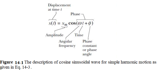
In Fig. 14-1 the argument of the cosine function is called the phase of the motion. The variation of phase with time, varies the value of the cosine function. The constant \(\phi\) is called the phase angle or phase constant.

The quantity \(\omega\) in Eq. 14-3 is the angular frequency of the motion and it is related to the frequency f and the period T. Let’s consider \(\omega=0\) in Eq. 14-3 to establish relation among \(\omega\), f and T by considering the period property of the cosine wave \(x(t) = x(t+T)\). Cosine wave returns to the same position can then be written as

\[\begin{equation} x_m\cos(\omega t) = x_m\cos\omega (t+T) \tag{14.4} \end{equation}\]

We can see in Eq.14-4 that the cosine function first repeats itself when its argument (the phase, remember) has increased by \(\phi = 2\pi\) rad. As a result we get

\[\omega(t+T)=\omega t + 2\pi\] \[\omega T = 2\pi\]

Therefore, the relation holding the relation between angular frequency \(\omega\), frequency f and time period T is established as follows:

\[\begin{equation} \omega = \frac{2\pi}{T} = 2\pi f \tag{14.5} \end{equation}\] The SI unit of angular frequency is the radian per second.

14.1.1 The Velocity and Acceleration of SHM

Now we want to observe how displacement of a sinusoidal wave as given in Eq. 14-3 relates to velocity and acceleration of the wave to establish Newton’s second law of motion.

We can the velocity v(t) as a function of time, by taking a time derivative of the position function x(t) in Eq. 14-3:

\[v(t)=\frac {dx(t)}{dt}=\frac{d}{dt}[x_m\cos(\omega t +\phi)]\]

\[\begin{equation} v(t) = -\omega x_m\sin(\omega t + \phi)=-v_m\sin(\omega t + \phi)~~~(velocity) \tag{14.6} \end{equation}\]

In Eq. 14-6, \(v_m = \omega x_m\), is the velocity amplitude of the velocity variation of the wave.

Similarly, if we take further derivative of Eq. 14-6, we get acceleration

\[a(t)=\frac {dv(t)}{dt}=\frac{d}{dt}[-\omega x_m\sin(\omega t +\phi)]\]

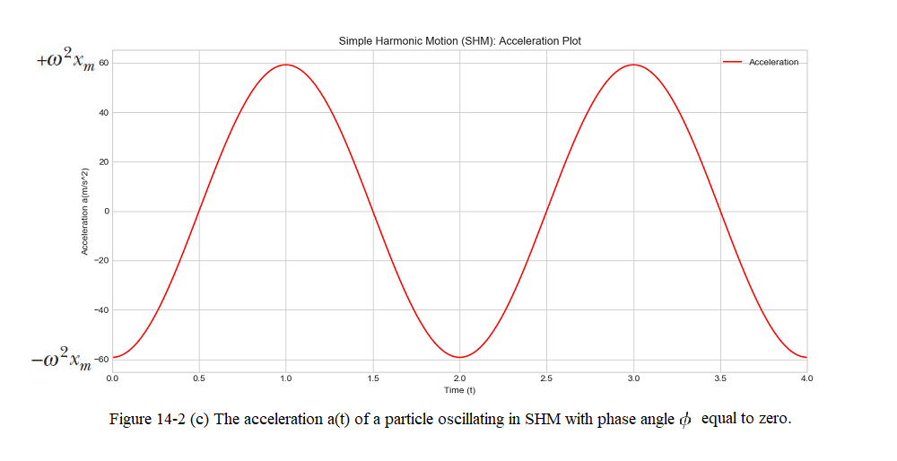
\[\begin{equation} a(t) = -\omega^2 x_m\cos(\omega t + \phi)= -a_m\cos(\omega t + \phi)~~~(acceleration) \tag{14.7} \end{equation}\]

In Eq. 14-7, \(a_m = \omega^2 x_m\), is the acceleration amplitude of the acceleration variation of the wave.

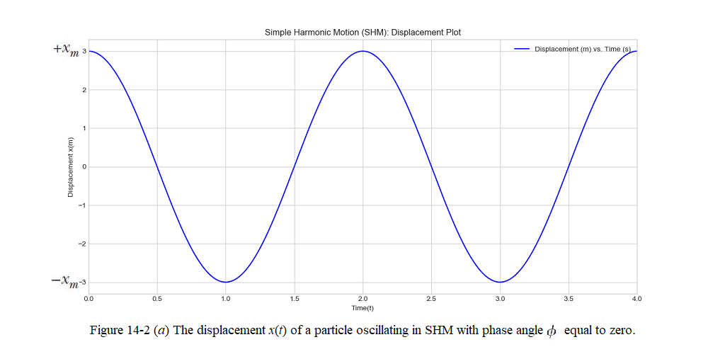
In Fig. 14-2, we can see the (a) the displacement x(t) of a particle oscillating in SHM with phase angle \(\phi\) equal to zero.The period T marks one complete oscillation. (b) The velocity v(t) of the particle. (c) The acceleration a(t) of the particle.

If we substitute Eq. 14-3 in Eq. 14-7, we can get the following reduced expression for acceleration

\[\begin{equation} a(t) = -\omega^2 x(t). \tag{14.8} \end{equation}\]

14.1.2 The Force Law for Simple Harmonic Motion:

We can apply Newton’s second law to find the force to generate the SHM. Using Eq. 14-8, we can find an expression for the acceleration in terms of the displacement as follows:

\[\begin{equation} F = ma = m(-\omega^2x) = -(m\omega^2)x \tag{14.9} \end{equation}\]

The minus sign in Eq. 14-9, indicates that the direction of the force on the particle is opposite to the direction of the displacement of the particle. The SHM is a restoring force meaning that fprce opposes the displacement, to restore the particle to the center point at x = 0.

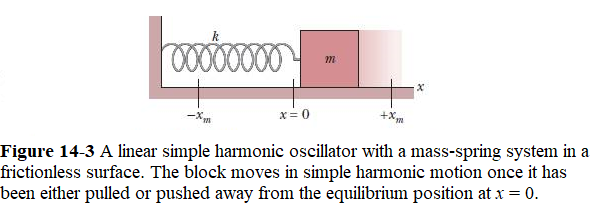
Now we apply the force in Eq. 14-9 to a block–spring system of Fig. 14-3 is called a linear simple harmonic oscillator (linear oscillator, for short), where linear indicates that F is proportional to x to the first power (and not to some other power).

The linear dependence of F is proportional to x we call it Hook’s law:

\[F = -kx\], where k is called the spring constant with SI unit is \(N/m\).

Combining Eq. 14-9 with Hook’s law \(F = -kx\), we get

\[\begin{equation} k = m\omega^2 \tag{14.10} \end{equation}\]

With a known oscillating mass, we can then determine the angular frequency of the motion from Eq. 15-10 as

\[\begin{equation} \omega = \sqrt\frac{k}{m}~~~(angular frequency). \tag{14.11} \end{equation}\]

Combining Eq. 14-5 and Eq. 14-12 we get the period of the SHM of the mass as follows:

\[\begin{equation} T = 2\pi\sqrt\frac{m}{k}~~~(period). \tag{14.12} \end{equation}\]

14.2 SHM) as the First Order Approximation:

Consider the motion of a point particle of mass \(m\) which is slightly displaced from a stable equilibrium point at \(x=0\). Suppose that the particle is moving in the conservative force-field \(F(x)\). In order for \(x=0\) to be a stable equilibrium point we require both

\[\begin{equation} F(0) = 0, \tag{14.13} \end{equation}\]

and

\[\begin{equation} \frac{d F(0)}{dx} < 0. \tag{14.14} \end{equation}\]

Now, our particle obeys Newton’s second law of motion,

\[\begin{equation} m\,\frac{d^2 x}{d t^2} = F(x). \tag{14.15} \end{equation}\]

Let us assume that it always stays fairly close to its equilibrium point. In this case, to a good approximation, we can represent \(F(x)\) via a truncated Taylor expansion about this point. In other words,

\[\begin{equation} F(x) \simeq F(0) + \frac{dF(0)}{dx}\,x + {\cal O}(x^2). \tag{14.16} \end{equation}\]

However, according to (14-9), the above expression can be written

\[\begin{equation} F(x) \simeq - m\,\omega_0^{\,2}\,x, \tag{14.17} \end{equation}\]

where \(dF(0)/dx = -m\,\omega_0^{\,2}\). Hence, we conclude that our particle satisfies the following approximate equation of motion,

\[\begin{equation} \frac{d^2 x}{dt^2}+ \omega_0^{\,2}\,x\simeq 0, \tag{14.18} \end{equation}\]

provided that it does not move too far from its equilibrium point: i.e., provided \(\vert x\vert\) does not become too large.

Equation (14-18) is called the simple harmonic equation, and governs the motion of all one-dimensional conservative systems which are slightly perturbed from some stable equilibrium state. The solution of Equation (14-18) is well-known as we considered in Eq. 14-3:

\[\begin{equation} x(t) = x_m\,\cos(\omega_0\,t + \phi_0). \tag{14.19} \end{equation}\]

The pattern of motion described by above expression, which is called simple harmonic motion, is periodic in time, with repetition period \(T_0 = 2\pi/\omega_0\), and oscillates between \(x=\pm x_m\). Here, \(x_m\) is called the amplitude of the motion. The parameter \(\phi_0\), known as the phase angle, simply shifts the pattern of motion backward and forward in time.

Note that the frequency, \(\omega_0\)–and, hence, the period, \(T_0\)–of simple harmonic motion is determined by the parameters appearing in the simple harmonic equation, (14-19). However, the amplitude, \(x_m\), and the phase angle, \(\phi_0\), are the two integration constants of this second-order ordinary differential equation, and are, thus, determined by the initial conditions: i.e., by the particle’s initial displacement and velocity.

Now, from Eq. 8-11 and Eq. 4-11, the potential energy of our particle at position \(x\) is approximately

\[\begin{equation} U(x) \simeq \frac{1}{2}\,m\,\omega_0^{\,2}\,x^2. \tag{14.20} \end{equation}\]

Hence, the total energy is written

\[\begin{equation} E = K + U = \frac{1}{2}\,m\left(\frac{dx}{dt}\right)^2+ \frac{1}{2}\,m\,\omega_0^{\,2}\,x^2, \tag{14.21} \end{equation}\]

giving

\[\begin{equation} E = \frac{1}{2}\,m\,\omega_0^{\,2}\,x_m^2\,\cos^2(\omega_0\,t-... ...n^2(\omega_0\,t-\phi_0) = \frac{1}{2}\,m\,\omega_0^{\,2}\,x_m^2, \tag{14.22} \end{equation}\]

where use has been made of Equation (14-8), and the trigonometric identity\(\cos^2\theta+\sin^2\theta \equiv 1\). Note that the total energy is constant in time, as is to be expected for a conservative system, and is proportional to the amplitude squared of the motion.

14.3 Damped Oscillatory Motion:

The SHM that we discusse in Equation (14-3) based on a one-dimensional conservative system theoretically oscillates about its equilibrium point with a fixed frequency and a constant amplitude without die down of the oscillations. But in reality, if we slightly perturb a dynamical system (such as a pendulum) from a stable equilibrium point then it will indeed oscillate about this point, but these oscillations will eventually die away due to frictional effects of air, which are present in virtually all real dynamical systems. To include the effect of damping in the system we consider a frictional drag force in our perturbed equation of motion, (14-18).

The most common model for a frictional drag force is one which is always directed in the opposite direction to the instantaneous velocity of the object upon which it acts, and is directly proportional to the magnitude of this velocity.

When the motion of an oscillator is reduced by an external force, the oscillator and its motion are said to be damped. An idealized example of a damped oscillator is shown in Fig. 14-4, where a block with mass m oscillates vertically on a spring with spring constant k. From the block, a rod extends to a vane (both assumed massless) that is submerged in a liquid.As the vane moves up and down, the liquid exerts an inhibiting drag force on it and thus on the entire oscillating system.With time, the mechanical energy of the block–spring system decreases, as energy is transferred to thermal energy of the liquid and vane.

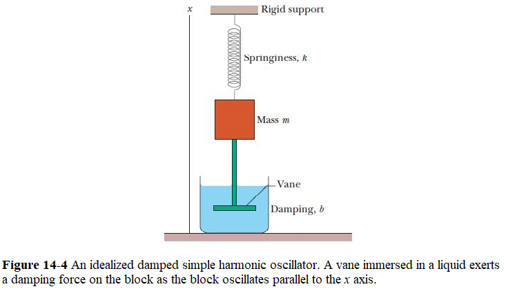
Let us adopt this model. So, our damping force can be written

\[\begin{equation} F_{d} =-b\frac{dx}{dt}, \tag{14.23} \end{equation}\]

where b is a damping constant that depends on the characteristics of both the vane and the liquid and has the SI unit of kilogram per second. The minus sign indicates that \(\vec F_d\) opposes the motion.

Damped Oscillations. The force on the block from the spring is \(F_s=-kx\). Let us assume that the gravitational force on the block is negligible relative to \(F_d\) and \(F_s\). Then we can write Newton’s second law for components along the x axis (\(F_{net,x}=ma_x\)) as

\[\begin{equation} -bv - kx = ma. \tag{14.24} \end{equation}\]

Substituting \(\frac{dx}{dt}\) for v and \(\frac{d^2x}{dt^2}\) for a and rearranging give us the differential equation

\[\begin{equation} m\frac{d^2 x}{dt^2} + b\frac{dx}{dt} + kx = 0. \tag{14.25} \end{equation}\]

Thus, the positive constant \(b\) parameterizes the strength of the frictional damping in our dynamical system. Equation (14-25) is a linear second-order ordinary differential equation. To solve Eq. 14-25, let us consider a trial solution of the form \(x(t) = x_m e^\nu t\), then we get

\[m\nu^2 + b\nu + k\] \[\nu^2+\frac{b}{m}\nu+\frac{k}{m}\] Solving quadratic equation, we get \[\nu=-\frac{b}{2m} \pm \sqrt{\frac{b^2}{4m^2}-\frac{k}{m}}\]

Therefore, the damped solution becomes,

\[\begin{equation} x = x_m e^{-\frac{bt}{2m}} e^{\pm i\omega't} =x_m e^{-\frac{bt}{2m}}\left(\cos\omega't \pm i\sin\omega't\right), \tag{14.26} \end{equation}\]

Taking the real part of Eq. 14-26, we get the solution of the damped oscillator as follows:

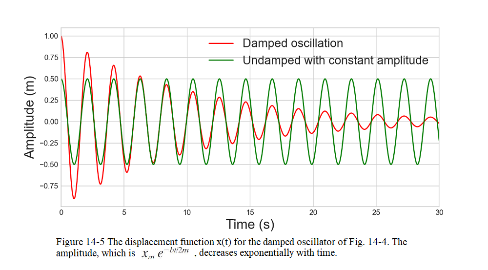
\[\begin{equation} x = x_m e^{-\frac{bt}{2m}}\left(\cos\omega't + \phi\right), \tag{14.27} \end{equation}\]

where \(\omega'=\sqrt{\frac{k}{m}-\frac{b^2}{4m^2}}\) is the angular frequeny of the damped oscillator.

If b = 0, we go back to undamped oscillator, with undamped angular frequency \(\omega = \sqrt\frac{k}{m}\) as given in Eq. 14-4 and the undamped solution \(x(t)=x_m\cos(\omega t + \phi)\). The sketch of Eq. 14-27 as shown in Fig. 14-5 shows the displacement function x(t) as a function of time of the damped oscillator.

14.4 Energy in Simple Harmonic Motion:

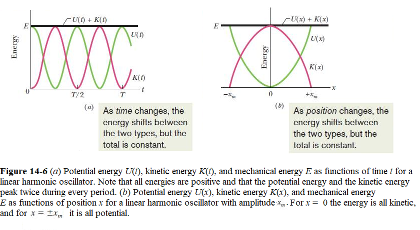
In SHM the energy transfers back and forth between kinetic energy and potential energy, while the sum of the two—the mechanical energy E of the oscillator—remains constant. The potential energy of a linear oscillator of a spring is shown in Fig. 14-6. The value of the potential energy of the spring depends on how much the spring is stretched or compressed— that is, on x(t). We can use Eqs. 8-5 and 14-3 to find the potential energy of the oscillator

\[\begin{equation} U(t) = \frac{1}{2}kx^2=\frac{1}{2}kx_m^2\cos^2(\omega t + \phi), \tag{14.28} \end{equation}\]

The kinetic energy of the system of Fig. 14-3 is associated entirely with the block. The value of the kinetic energy depends on how fast the block is moving—that is, on v(t) as derived in Eq. 14-4

\[\begin{equation} K(t) = \frac{1}{2}mv^2=\frac{1}{2}m\omega^2 x_m^2\sin^2(\omega t + \phi), \tag{14.29} \end{equation}\]

Using Eq. 14-11, we can rewrite Eq. 14-29 as follows

\[\begin{equation} K(t) =\frac{1}{2}kx_m^2\sin^2(\omega t + \phi), \tag{14.30} \end{equation}\]

The mechanical energy is the sum of potential and kinetic energies as derived in Eqs. 14-28 and 14-30 as

\[\begin{equation} E(t) =\frac{1}{2}kx_m^2\sin^2(\omega t + \phi)+\frac{1}{2}kx_m^2\cos^2(\omega t + \phi)=\frac{1}{2}kx_m^2, \tag{14.31} \end{equation}\]

The mechanical energy of a linear oscillator is constant and independent of time. The potential energy, kinetic energy and mechanical energy of a linear oscillator are shown as functions of time t in Fig. 14-6a and as functions of displacement x in Fig. 14-6b.

14.5 Quality Factor:

The total mechanical energy of a damped oscillator is the sum of its kinetic and potential energies,

\[\begin{equation} E = \frac{1}{2}\,m\left(\frac{dx}{dt}\right)^2 + \frac{1}{2}\,m\,\omega_0^{\,2}\,x^2. \tag{14.32} \end{equation}\]

Differentiating the above expression with respect to time, we obtain

\[\begin{equation} \frac{dE}{dt} = m\frac{dx}{dt}\frac{d^2 x}{dt^2} + m\omega_0^2x\frac{dx}{dt}=m\frac{dx}{dt}\left(\frac{d^2 x}{dt^2} + \omega_0^{\,2}\,x\right). \tag{14.33} \end{equation}\]

\[\begin{equation} f_{drag} = - 2\,m\,\nu\,\frac{dx}{dt}, \tag{14.34} \end{equation}\]

where \(\nu\) is a positive constant with the dimensions of frequency. Including such a force in our perturbed equation of motion, Eq. 14-18, we obtain

\[\begin{equation} \frac{d^2 x}{dt^2} + 2\,\nu\,\frac{dx}{dt} + \omega_0^{\,2}\,x = 0. \tag{14.35} \end{equation}\]

It follows from Eq. 14-35 that \[\begin{equation} \frac{dE}{dt} = -2\,m\,\nu\left(\frac{dx}{dt}\right)^2. \tag{14.36} \end{equation}\]

The energy loss rate of a weakly damped (i.e.,\(\nu\ll\omega_0\)) oscillator is conveniently characterized in terms of a parameter, \(Q\), which is known as the quality factor. This parameter is defined to be \(2\pi\) times the energy stored in the oscillator, divided by the energy lost in a single oscillation period. If the oscillator is weakly damped then the energy lost per period is relatively small, and \(Q\) is therefore much larger than unity. Roughly speaking, \(Q\) is the number of oscillations that the oscillator typically completes, after being set in motion, before its amplitude decays to a negligible value. Let us find an expression for \(Q\).

Now, the most general solution for a weakly damped oscillator can be written in the form [cf., Equation (91)]

\[\begin{equation} x = x_0\,{\rm e}^{-\nu\,t}\,\cos(\omega_r\,t-\phi_0), \tag{14.37} \end{equation}\]

where \(x_0\) and \(\phi_0\) are constants, and \(\omega_r = \sqrt{\omega_0^{\,2}-\nu^2}\). It follows that

\[\begin{equation} \frac{dx}{dt} =- x_0\nu {\rm e}^{-\nu t}\cos(\omega_r t-\phi_0)- x_0\omega_r\,{\rm e}^{-\nu t}\sin(\omega_r t-\phi_0). \tag{14.38} \end{equation}\]

Thus, making use of Eq. 14-36, the energy lost during a single oscillation period is

\[\begin{equation} \Delta E =-\int_0^{T_r} \frac{dE}{dt}\,dt = 2\,m\,\nu\,x_0^{\,2}\int_0^{T_r}{\rm e}^{-2\,\nu\,t}\left[\nu\,\cos(\omega_r\,t-\phi_0) + \omega_r\,\sin(\omega_r\,t-\phi_0)\right]^2 dt, \end{equation}\]

where \(T_r=2\pi/\omega_r\). In the weakly damped limit, \(\nu\ll \omega_r\), the exponential factor is approximately unity in the interval \(t=0\) to \(t=T_r\), so that

\[\begin{equation} \Delta E \simeq \frac{2\,m\,\nu\,x_0^{\,2}}{\omega_r}\int_0^{2\pi}\left(\nu^2\cos^2\theta+2\nu\omega_r\cos^2\theta\sin\theta + \omega_r^{\,2}\,\sin^2\theta\right)d\theta. \end{equation}\]

Thus, \[\begin{equation} \Delta E \simeq \frac{2\pi\,m\,\nu\,x_0^{\,2}}{\omega_r}\,(\nu^2+\omega_r^{\,2}) =2\pi m\omega_0^2,x_0^{\,2}\left(\frac{\nu}{\omega_r}\right), \end{equation}\]

since \(\cos^2\theta\) and \(\sin^2\theta\) both have the average values \(1/2\) in the interval \(0\) to \(2\pi\), whereas \(\cos\theta\,\sin\theta\) has the average value \(0\). According to Eq. 14-22, the energy stored in the oscillator (at \(t=0\)) is

\[\begin{equation} E = \frac{1}{2}\,m\,\omega_0^{\,2}\,x_0^{\,2}. \end{equation}\]

It follows that

\[\begin{equation} Q = 2\pi\,\frac{E}{\Delta E} = \frac{\omega_r}{2\,\nu}\simeq \frac{\omega_0}{2\,\nu}. \tag{14.39} \end{equation}\]

14.6 Resonance:

We have seen that when a one-dimensional dynamical system is slightly perturbed from a stable equilibrium point (and then left alone), it eventually returns to this point at a rate controlled by the amount of damping in the system. Let us now suppose that the same system is subject to continuous oscillatory constant amplitude external driving force at some fixed frequency, \(\omega\). In this case, we would expect the system to eventually settle down to some steady oscillatory pattern of motion with the same frequency as the external force. Let us investigate the properties of this type of driven oscillation. Suppose that our system is subject to an external force of the form

\[\begin{equation} f_{ext}(t) = m\,\omega_0^{\,2}\,X_1\,\cos(\omega\,t). \tag{14.40} \end{equation}\]

Here, \(X_1\) is the amplitude of the oscillation at which the external force matches the restoring force, Eq. 14-17. Incorporating the above force into our perturbed equation of motion, Eq.14-35, we obtain

\[\begin{equation} \frac{d^2 x}{dt^2} + 2\,\nu\,\frac{dx}{dt} + \omega_0^{\,2}\,x = \omega_0^{\,2}\,X_1\,\cos(\omega\,t). \tag{14.41} \end{equation}\]

Let us search for a solution to represent the right-hand side of the above equation as

\(\omega_0^{\,2}\,X_1\,\exp(-{\rm i}\,\omega\,t)\). It is again understood that the physical solutions are the real parts of these expressions. Note that \(\omega\) is now a real parameter. We obtain

\[\begin{equation} \alpha\left[-\omega^2-{\rm i}\,2\,\nu\,\omega + \omega_0^{\,2}\right]{\rm e}^{-{\rm i}\,\omega\,t} = \omega_0^{\,2}\,X_1\,{\rm e}^{-{\rm i}\,\omega\,t}. \tag{14.42} \end{equation}\]

Hence, \[\begin{equation} \alpha = \frac{\omega_0^{\,2}\,X_1}{\omega_0^{\,2}-\omega^2 - {\rm i}\,2\,\nu\,\omega}. \tag{14.43} \end{equation}\]

In general, \(a\) is a complex quantity. Thus, we can write

\[\begin{equation} \alpha = x_1\,{\rm e}^{\,{\rm i}\,\phi_1}, \tag{14.44} \end{equation}\]

where \(x_1\) and \(\phi_1\) are both real. It follows from Equations (84), (107), and (108) that the physical solution takes the form

\[\begin{equation} x(t) = x_1\,\cos(\omega\,t-\phi_1), \tag{14.45} \end{equation}\]

where

\[\begin{equation} x_1 = \frac{\omega_0^{\,2}\,X_1}{\left[(\omega_0^{\,2}-\omega^2)^2 + 4\,\nu^2\,\omega^2\right]^{1/2}}, \tag{14.46} \end{equation}\]

\[\begin{equation} \frac{x_1}{X_1} = \frac{1}{\left[(1-\frac{\omega^2}{\omega_0^2})^2 + \frac{4\,\nu^2\,\omega^2}{\omega_0^2}\right]^{1/2}}, \tag{14.47} \end{equation}\]

and

\[\begin{equation} \phi_1 = \tan^{-1}\left(\frac{2\,\nu\,\omega}{\omega_0^{\,2}-\omega^2}\right). \tag{14.48} \end{equation}\]

We conclude that, in response to the applied sinusoidal force, Eq.14-40, the system executes a sinusoidal pattern of motion at the same frequency, with fixed amplitude \(x_1\), and phase-lag \(\phi_1\) (with respect to the external force) as shown in Fig. 14-7

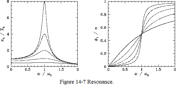
Let us investigate the variation of \(x_1\) and \(\phi_1\) with the forcing frequency, \(\omega\). This is most easily done graphically. Fig. 14-7 shows \(x_1\) and \(\phi_1\) as functions of \(\omega\) for various values of \(\nu/\omega_0\). Here, \(\nu/\omega_0 = 1\), \(1/2\), \(1/4\), \(1/8\), and \(1/16\) correspond to the solid, dotted, short-dashed, long-dashed, and dot-dashed curves, respectively. It can be seen that as the amount of damping in the system is decreased, the amplitude of the response becomes progressively more peaked at the natural frequency of oscillation of the system, \(\omega_0\). This effect is known as resonance, and \(\omega_0\) is termed the resonant frequency. Thus, a weakly damped system (i.e., \(\nu\ll\omega_0\)) can be driven to large amplitude by the application of a relatively small external force which oscillates at a frequency close to the resonant frequency. Note that the response of the system is in phase (i.e., \(\phi_1\simeq 0\)) with the external driving force for driving frequencies well below the resonant frequency, is in phase quadrature (i.e., \(\phi_1=\pi/2\)) at the resonant frequency, and is in anti-phase (i.e., \(\phi_1\simeq \pi\)) for frequencies well above the resonant frequency. According to Eq.14-46,

\[\begin{equation} \frac{x_1(\omega=\omega_0)}{x_1(\omega = 0)} = \frac{\omega_0}{2\,\nu} =Q. \tag{14.49} \end{equation}\]

In other words, the ratio of the driven amplitude at the resonant frequency to that at a typical non-resonant frequency (for the same drive amplitude) is of order the quality factor. Eq. 14-46 also implies that, for a weakly damped oscillator ( \(\nu\ll\omega_0\)),

\[\begin{equation} \frac{x_1(\omega)}{x_1(\omega=\omega_0)}\simeq \frac{\nu}{[(\omega-\omega_0)^2 + \nu^2]^{1/2}}, \tag{14.50} \end{equation}\]

provided \(\vert\omega-\omega_0\vert\ll \omega_0\). Hence, the width of the resonance peak (in frequency) is \(\Delta\omega = 2\,\nu\), where the edges of peak are defined as the points at which the driven amplitude is reduced to \(1/\sqrt{2}\) of its maximum value. It follows that the fractional width is

\[\begin{equation} \frac{\Delta \omega}{\omega_0} = \frac{2\,\nu}{\omega_0} = \frac{1}{Q}. \tag{14.51} \end{equation}\]

We conclude that the height and width of the resonance peak of a weakly damped (\(Q\gg 1\)) oscillator scale as \(Q\) and \(Q^{-1}\), respectively. Thus, the area under the resonance curve stays approximately constant as \(Q\) varies.

14.7 Periodic Driving Forces:

In the last section, we investigated the response of a one-dimensional dynamical system, close to a stable equilibrium point, to an external force which varies as \(\cos(\omega\,t)\). Let us now examine the response of the same system to a more complicated external force.

Consider a general external force which is periodic in time, with period \(T\). By analogy with Eq. 14-40, we can write such a force as

\[\begin{equation} f_{ext}(t) = m\,\omega_0^{\,2}\,X(t), \tag{14.52} \end{equation}\]

where

\[\begin{equation} X(t+T) = X(t) \tag{14.53} \end{equation}\]

for all \(t\). It is convenient to represent \(X(t)\) as a Fourier series in time, so that

\[\begin{equation} X(t) = \sum_{n=0}^{\infty} X_{n}\,\cos(n\,\omega\,t), \tag{14.54} \end{equation}\]

where \(\omega = 2\pi/T\). By writing \(X(t)\) in this form, we automatically satisfy the periodicity constraint Eq.14-53. [Note that by choosing a cosine Fourier series we are limited to even functions in \(t\): i.e., \(X(-t)=X(t)\). Odd functions in \(t\) can be represented by sine Fourier series, and mixed functions require a combination of cosine and sine Fourier series.] The constant coefficients \(X_n\) are known as Fourier coefficients. But, how do we determine these coefficients for a given functional form, \(X(t)\)? Well, it follows from the periodicity of the cosine function that

\[\begin{equation} \frac{1}{T} \int_0^T \cos (n\,\omega\,t)\,dt = \delta_{n\,0}, \tag{14.55} \end{equation}\]

where \(\delta_{n\,n'}\) is unity if \(n=n'\), and zero otherwise, and is known as the Kronecker delta function. Thus, integrating Eq. 14-54 in \(t\) from \(t=0\) to \(t=T\), and making use of Eq. 14-55, we obtain

\[\begin{equation} X_0 = \frac{1}{T}\int_0^T X(t) \,dt. \tag{14.56} \end{equation}\]

It is also easily demonstrated that

\[\begin{equation} \frac{2}{T} \int_0^T \cos(n\,\omega\,t)\,\cos(n'\,\omega\,t) \,dt= \delta_{n\,n'}, \tag{14.57} \end{equation}\]

provided \(n, n'>0\). Thus, multiplying Eq. 14-54 by \(\cos(n\,\omega\,t)\), integrating in \(t\) from \(t=0\) to \(t=T\), and making use of Eq. 14-55 and Eq. , we obtain

\[\begin{equation} X_n = \frac{2}{T} \int_0^T X(t)\,\cos(n\,\omega\,t)\,dt \tag{14.58} \end{equation}\]

for \(n>0\). Hence, we have now determined the Fourier coefficients of the general periodic function \(X(t)\). We can incorporate the periodic external force Eq.14-52 into our perturbed equation of motion by writing

\[\begin{equation} \frac{d^2 x}{dt^2} + 2\,\nu\,\frac{dx}{dt} +\omega_0^{\,2}x= \omega_0^{\,2}\sum_{n=0}^\infty X_n\,{\rm e}^{-{\rm i}\,n\,\omega\,t}, \tag{14.58} \end{equation}\]

where we are again using the convention that the physical solution corresponds to the real part of the complex solution. Note that the above differential equation is linear. This means that if \(x_a(t)\) and \(x_b(t)\) represent two independent solutions to this equation then any linear combination of \(x_a(t)\) and \(x_b(t)\) is also a solution. We can exploit the linearity of the above equation to write the solution in the form

\[\begin{equation} x(t) = \sum_{n=0}^\infty X_n\,a_n\,{\rm e}^{-{\rm i}\,n\,\omega\,t}, \tag{14.59} \end{equation}\]

where the \(a_n\) are the complex amplitudes of the solutions to

\[\begin{equation} \frac{d^2 x}{dt^2} + 2\,\nu\,\frac{dx}{dt} + \omega_0^{\,2}\,x = \omega_0^{\,2}\,{\rm e}^{-{\rm i}\,n\,\omega\,t}. \tag{14.60} \end{equation}\]

In other words, \(a_n\) is obtained by substituting \(x = a_n\,\exp(-{\rm i}\,n\,\omega\,t)\) into the above equation. Hence, it follows that

\[\begin{equation} a_n = \frac{\omega_0^{\,2}}{\omega_0^{\,2} - n^2\,\omega^2 - {\rm i}\,2\,\nu\,n\,\omega}. \tag{14.61} \end{equation}\]

Thus, the physical solution takes the form

\[\begin{equation} x(t) = \sum_{n=0}^{\infty} X_n\,x_n\,\cos(n\,\omega\,t-\phi_n), \tag{14.62} \end{equation}\]

where

\[\begin{equation} a_n = x_n \,{\rm e}^{\,{\rm i}\,\phi_n}, \tag{14.63} \end{equation}\]

and \(x_n\) and \(\phi_n\) are real parameters. It follows from Eq. 14-61 that

\[\begin{equation} x_n = \frac{\omega_0^{\,2}}{\left[(\omega_0^{\,2}-n^2\,\omega^2)^2 + 4\,\nu^2\,n^2\,\omega^2\right]^{1/2}}, \tag{14.64} \end{equation}\]

and

\[\begin{equation} \phi_n = \tan^{-1}\left(\frac{2\,\nu\,n\,\omega}{\omega_0^{\,2}-n^2\,\omega^2}\right). \tag{14.65} \end{equation}\]

We have now fully determined the response of our dynamical system to a general periodic driving force. As an example, suppose that the external force periodically delivers a brief kick to the system. For instance, let \(X(t) = A\) for \(0\leq t\leq T/10\) and \(9\,T/10<t<T\), and \(X(t)=0\) otherwise (in the period \(0\leq t\leq T\)). It follows from Eq.14-56 and 14-58 that, in this case,

\[\begin{equation} X_0 = 0.2\,A, \tag{14.66} \end{equation}\]

and

\[\begin{equation} X_n = \frac{2\,\sin(n\,\pi/5)\,A}{n\,\pi}, \tag{14.67} \end{equation}\]

for \(n>0\). Obviously, to obtain an exact solution, we would have to include every Fourier harmonic in Eq. 14-62, which would be impractical. However, we can obtain a fairly accurate approximate solution by truncating the Fourier series (i.e., by neglecting all the terms with \(n>N\), where \(N\gg 1\)).

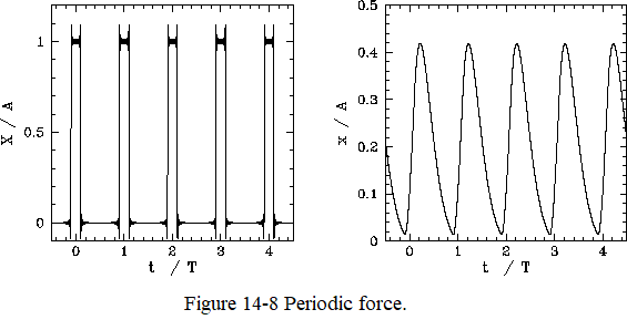
Figure 14-8 shows an example calculation in which the Fourier series is truncated after 100 terms. The parameters used in this calculation are \(\omega = 1.2\,\omega_0\) and \(\nu= 0.8\,\omega_0\). The left panel shows the Fourier reconstruction of the driving force, \(X(t)\). The glitches at the rising and falling edges of the pulses are called Gibbs phenomena, and are an inevitable consequence of attempting to represent a discontinuous periodic function as a Fourier series. The right panel shows the Fourier reconstruction of the response, \(x(t)\), of the dynamical system to the applied force.

14.8 Transients:

We saw, in Section 3.7, that when a one-dimensional dynamical system, close to a stable equilibrium point, is subject to a sinusoidal external force of the form Eq. 14-40 then the equation of motion of the system is written

\[\begin{equation} \frac{d^2 x}{dt^2} + 2\,\nu\,\frac{dx}{dt} + \omega_0^{\,2}\,x = \omega_0^{\,2}\,X_1\,\cos(\omega\,t). \tag{14.68} \end{equation}\]

We also found that the solution to this equation which oscillates in sympathy with the applied force takes the form

\[\begin{equation} x(t) = x_1\,\cos(\omega\,t-\phi_1), \tag{14.69} \end{equation}\]

where \(x_1\) and \(\phi_1\) are specified in Eq. 14-46 and Eq. 14-48, respectively. However, Eq. 14-69 is not the most general solution to Eq. 14-68. It should be clear that we can take the above solution and add to it any solution of Eq. 14-68 calculated with the right-hand side set to zero, and the result will also be a solution of Eq. 14-68. Now, we investigated the solutions to Eq. 14-68 with the right-hand set to zero in Section 3.5. In the underdamped regime (\(\nu < \omega_0\)), we found that the most general such solution takes the form

\[\begin{equation} x(t) = A\,{\rm e}^{-\nu\,t}\,\cos(\omega_r\,t) + B\,{\rm e}^{-\nu\,t}\, \sin(\omega_r\,t), \tag{14.69} \end{equation}\]

where \(A\) and \(B\) are two arbitrary constants [they are in fact the integration constants of the second-order ordinary differential Eq. 14-68], and \(\omega_r = \sqrt{\omega_0^{\,2}-\nu^2}\). Thus, the most general solution to Eq. 14-68 is written

\[\begin{equation} x(t) = A\,{\rm e}^{-\nu\,t}\,\cos(\omega_r\,t) + B\,{\rm e}^{-\nu\,t}\, \sin(\omega_r\,t) + x_1\,\cos(\omega\,t-\phi_1). \tag{14.70} \end{equation}\]

The first two terms on the right-hand side of the above equation are called transients, since they decay in time. The transients are determined by the initial conditions. However, if we wait long enough after setting the system into motion then the transients will always decay away, leaving the time-asymptotic solution Eq. 14-69, which is independent of the initial conditions.

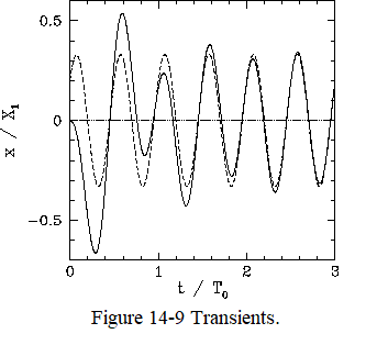
As an example, suppose that we set the system into motion at time \(t=0\) with the initial conditions \(x(0)=dx(0)/dt=0\). Setting \(x(0)=0\) in Eq. 14-70, we obtain

\[\begin{equation} A = - x_1\,\cos\phi_1. \tag{14.71} \end{equation}\]

Moreover, setting \(dx(0)/dt=0\) in Eq. 14-70, we get

\[\begin{equation} B = -\frac{x_1\,(\nu\,\cos\phi_1+\omega\,\sin\phi_1)}{\omega_r}. \tag{14.72} \end{equation}\]

Thus, we have now determined the constants \(A\) and \(B\), and, hence, fully specified the solution for \(t>0\). Figure 8 shows this solution (solid curve) calculated for \(\omega = 2\,\omega_0\) and \(\nu=0.2\,\omega_0\). Here, \(T_0 = 2\pi/\omega_0\). The associated time-asymptotic solution Eq. 14-69 is also shown for the sake of comparison (dashed curve). It can be seen that the full solution quickly converges to the time-asymptotic solution.

14.9 Simple Pendulum:

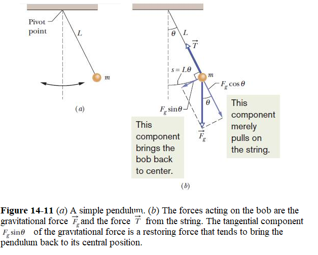
Let us consider a simple pendulum, which consists of a particle of mass m (called the bob of the pendulum) suspended from one end inextensible massless string of length \(L\), which is fixed at the other end, as in Fig. 14-11a.The bob is free to swing back and forth in the plane of the page, to the left and right of a vertical line through the pendulum’s pivot point. The Restoring Torque.

The forces acting on the bob are the force \(\vec T\) from the string and the gravitational force \(\vec F_g\), as shown in Fig. 14-11b, where the string makes an angle \(\theta\) with the vertical. The stable equilibrium state of the simple pendulum corresponds to the position in which the mass is stationary, and hangs vertically down with \(\theta=0\)). We resolve \(\vec F_g\) into a radial component \(F_g\cos\theta\) and a component \(F_g \sin\theta\) that is tangent to the path taken by the bob.This tangential component produces a restoring torque about the pendulum’s pivot point because the component always acts opposite the displacement of the bob so as to bring the bob back toward its central location. That location is called the equilibrium position \(\theta=0\)) because the pendulum would be at rest there were it not swinging.

The two forces acting on the mass are the downward gravitational force, \(m\,g\), where \(g\) is the acceleration due to gravity, and the tension, \(T\), in the string. Note, however, that the tension makes no contribution to the torque, since its line of action clearly passes through the pivot point. From simple trigonometry, the line of action of the gravitational force passes a distance \(l\,\sin\theta\) from the pivot point. Hence, the magnitude of the gravitational torque is \(m\,g\,l\, \sin\theta\). Moreover, the gravitational torque is a restoring torque: i.e., if the mass is displaced slightly from its equilibrium state (i.e., \(\theta=0\)) then the gravitational torque clearly acts to push the mass back toward that state. Thus, we can write

\[\begin{equation} \tau = - m\,g\,l\,\sin\theta. \tag{14.73} \end{equation}\]

From Newton’s second law for rotation \(\tau = I\alpha=I\frac{d^2{\theta}}{dt^2}\), the angular equation of motion of the pendulum is

\[\begin{equation} I\,\frac{d^2{\theta}}{dt^2} = \tau, \tag{14.74} \end{equation}\]

where \(I\) is the moment of inertia of the mass (see Section 8.3), and \(\tau\) is the torque acting about the pivot point (see Section A.7). For the case in hand, given that the mass is essentially a point particle, and is situated a distance \(L\) from the axis of rotation (i.e., the pivot point), it is easily seen that \(I=m\,L^2\).

Combining the previous two equations, we obtain the following angular equation of motion of the pendulum:

\[\begin{equation} L\,\frac{d^2{\theta}}{dt^2} +g\,\sin\theta=0. \tag{14.75} \end{equation}\]

Eq.14-75 is nonlinear [since \(\sin(a\,\theta)\neq a\,\sin\theta\), except for small angle when \(\theta\ll 1\).

In the small angle approximation or assuming the oscillations not far from its equilibrium state (\(\theta=0\)). We can keep the first term of the Tayor series expansion of \(\sin\theta\simeq \theta\), and the above equation of motion simplifies to

\[\begin{equation} \frac{d^2\theta}{dt^2} + \omega_0^{\,2}\,\theta\simeq 0, \tag{14.76} \end{equation}\]

where \(\omega_0 = \sqrt{g/L}=\sqrt{mgL/I}\), with \(I = mL^2\). Of course, this is just the simple harmonic equation which we discussed in the earlier sections. The solution of this equation is

\[\begin{equation} \theta(t) = \theta_0\,\cos(\omega_0\,t). \tag{14.77} \end{equation}\]

So, the pendulum swings back and forth at a fixed frequency, \(\omega_0\), which depends on \(L\) and \(g\), but is independent of the amplitude, \(\theta_0\), of the motion.

Suppose, we wish to look for a more accurate solution of Eq. 14-76. One way in which we could achieve this would be to include more terms in the small angle expansion of \(\sin\theta\), which is

\[\begin{equation} \sin\theta = \theta - \frac{\theta^{\,3}}{3!} + \frac{\theta^{\,5}}{5!} +\cdots. \tag{14.78} \end{equation}\]

Considering the first two terms in this expansion, Eq. 14-76 becomes

\[\begin{equation} \frac{d^2\theta}{dt^2} + \omega_0^{\,2}\,(\theta-\theta^{\,3}/6)\simeq 0. \tag{14.79} \end{equation}\]

Let us try a trial solution of the form of Eq. 14-77

\[\begin{equation} \theta(t) = \vartheta_0\,\cos(\omega\,t). \tag{14.80} \end{equation}\]

Substituting this into Eq.14-79, and making use of the following trigonometric identity

\[\begin{equation} \cos^3 u \equiv (3/4)\,\cos u+ (1/4)\,\cos(3\,u), \tag{14.81} \end{equation}\]

we obtain

\[\begin{equation} \vartheta_0\left[\omega_0^{\,2}-\omega^2 - (1/8)\omega_0^{\,2} \vartheta_0^{\,2}\right]\cos(\omega\,t)-(1/24)\omega_0^{\,2}\vartheta_0^{\,3} \cos(3\omega\,t)\simeq 0. \tag{14.82} \end{equation}\]

It is evident that the above equation cannot be satisfied for all values of \(t\), except in the trivial case \(\vartheta_0=0\). However, the form of this expression does suggest a better trial solution, namely

\[\begin{equation} \theta(t) = \vartheta_0\,\cos(\omega\,t) + \alpha\,\vartheta_0^{\,3}\,\cos(3\,\omega\,t), \tag{14.83} \end{equation}\]

where \(\alpha\) is \({\cal O}(1)\). Substitution of this expression into Eq. 14-79 yields

\[\begin{equation} \vartheta_0\left[\omega_0^{\,2}-\omega^2 - (1/8)\,\omega_0^{\,2}\,\vartheta_0^{\,2} \right] \cos(\omega\,t) + \vartheta_0^{\,3}\left[\alpha\,\omega_0^{\,2} - 9\,\alpha\,\omega^2- (1/24)\,\omega_0^{\,2}\right] \cos(3\,\omega\,t) + {\cal O}(\vartheta_0^{\,5}) \simeq 0. \tag{14.84} \end{equation}\]

We can only satisfy the above equation at all values of \(t\), and for non-zero \(\vartheta_0\), by setting the two expressions in square brackets to zero. This yields

\[\begin{equation} \omega \simeq \omega_0 \,\sqrt{1-(1/8)\,\vartheta_0^{\,2}}, \tag{14.85} \end{equation}\]

and

\[\begin{equation} \alpha\simeq -\frac{\omega_0^{\,2}}{192}. \tag{14.86} \end{equation}\]

Now, the amplitude of the motion is given by

\[\begin{equation} \theta_0 = \vartheta_0 + \alpha\,\vartheta_0^{\,3} = \vartheta_0-\frac{\omega_0^{\,2}}{192}\,\vartheta_0^{\,3}. \tag{14.87} \end{equation}\]

Hence, Eq.14-85 simplifies to

\[\begin{equation} \omega = \omega_0\left[1-\frac{\theta_0^{\,2}}{16} + {\cal O}(\theta_0^{\,4})\right]. \tag{14.88} \end{equation}\]

The above expression is only approximate, but it illustrates an important point: i.e., that the frequency of oscillation of a simple pendulum is not, in fact, amplitude independent. Indeed, the frequency goes down slightly as the amplitude increases.

The above example illustrates how we might go about solving a nonlinear equation of motion by means of an expansion in a small parameter (in this case, the amplitude of the motion).

14.10 The Physical Pendulum:

A real pendulum as in Figure 14-12 shows an arbitrary physical pendulum displaced to one side by angle \(\theta\).

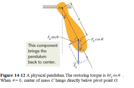
The gravitational force \(\vec F_g\) acts at its center of mass C, at a distance h from the pivot point O. Comparison of Figs. 14-12 and 14-11b reveals only one important difference between an arbitrary physical pendulum and a simple pendulum. For a physical pendulum the restoring component \(F_g \sin\theta\) of the gravitational force has a moment arm of distance h about the pivot point, rather than of string length L. In all other respects, an analysis of the physical pendulum would duplicate our analysis of the simple pendulum. Again (for small \(\theta_m\)), we would find that the motion is approximately SHM. Let us start considering Eq. 14-76, with

\[\begin{equation} \omega = \sqrt{mgh/I} \tag{14.89}, \end{equation}\]

where we have replaced L with h, we can then write the period as

\[\begin{equation} T= \sqrt{I/mgh}~~~(physical~ pendulum, small ~amplitude). \tag{14.90}, \end{equation}\]

Similar to the simple pendulum, I is the rotational inertia of the pendulum about O. However, now I is not simply \(mL^2\) (it depends on the shape of the physical pendulum), but it is still proportional to m. A physical pendulum will not swing if it pivots at its center of mass. Formally, this corresponds to putting \(h = 0\) in Eq. 14-90.That equation then predicts \(T \to \infty\), which implies that such a pendulum will never complete one swing.

Corresponding to any physical pendulum that oscillates about a given pivot point O with period T is a simple pendulum of length \(L_0\) with the same period T. We can find \(L_0\) with Eq. 15-28.The point along the physical pendulum at distance \(L_0\) from point O is called the center of oscillation of the physical pendulum for the given suspension point.

We can use a physical pendulum to measure the free-fall acceleration g at a particular location on Earth’s surface. To analyze a simple case, take the pendulum to be a uniform rod of length L, suspended from one end. For such a pendulum, h in Eq. 15-29, the distance between the pivot point and the center of mass, is L.Table 10-2e tells us that the rotational inertia of this pendulum about a perpendicular axis through its center of mass is \(mL^2\). From the parallel-axis theorem of Eq. 10-36 \(\left(I=I_{com}+Mh^2\right)\), we then find that the rotational inertia about a perpendicular axis through one end of the rod is

\[\begin{equation} I = I_{com}+Mh^2 = \frac{1}{12}mL^2+m(\frac{1}{2}L)^2=\frac{1}{3}mL^2 \tag{14.91}, \end{equation}\]

If we put \(h = L\) and \(I =\frac{1}{3} mL^2\) in Eq. 14-90 and solve for g, we find

\[\begin{equation} g = \frac{8\pi^2L}{3T^2} \tag{14.92}, \end{equation}\]

Thus, by measuring L and the period T, we can find the value of g at the pendulum’s location.

(Solved Problems : 11, 22, 24, 25, 33, 34, 59, 61)