Chapter-1 Fundamentals of Engineering (FE):

The Fundamentals of Engineering (FE) examination is one of four steps to be completed toward registering as a Professional Engineer (PE).

The Fundamentals of Engineering (FE) exam is generally the first step in the process to becoming a professional licensed engineer (P.E.). It is designed for recent graduates and students who are close to finishing an undergraduate engineering degree from an EAC/ABET-accredited program. The FE exam is a computer-based exam administered year-round at NCEES-approved Pearson VUE test centers.

The FE exam includes 110-questions. The exam appointment time is 6 hours long and includes:

Nondisclosure agreement (2 minutes)
Tutorial (8 minutes)
Exam (5 hours and 20 minutes)
Scheduled break (25 minutes)

Register for an FE exam by logging in to your MyNCEES account and following the onscreen instructions. Prepare for the FE exam by

Reviewing the FE exam specifications, fees, and requirements
Reading the reference materials
Understanding scoring and reporting

A $175 exam fee is payable directly to NCEES. Some licensing boards may require you to file a separate application and pay an application fee as part of the approval process to qualify you for a seat for an NCEES exam. Your licensing board may have additional requirements.

Exam specifications

The FE is offered in seven disciplines. Specifications for each discipline are as follows:

FE Chemical
FE Civil
FE Electrical and Computer
FE Environmental
FE Industrial and Systems
FE Mechanical
FE Other Disciplines

The computer-based FE contains alternative item types (AITs). AITs are questions other than traditional multiple-choice questions.

Each of the 50 states in the United States has laws that regulate the practice of engineering; these laws are designed to ensure that registered professional engineers have demonstrated sufficient competence and experience. The same exam is administered at designated times throughout the country, but each state’s Board of Registration administers the exam and supplies information and registration forms. Additional information is available on the NCEES website.

Four steps are required to become a Professional Engineer (PE):

Education. Usually this requirement is satisfied by completing a B.S. degree in engineering from an accredited college or university.
Fundamentals of Engineering examination. One must pass an 8-hour examination described in Section D.2.
Experience. Following successful completion of the Fundamentals of Engineering examination, two to four years of engineering experience are required.
Principles and practices of engineering examination. One must pass a second 8-hour examination, also known as the Professional Engineer (PE) examination, which requires in-depth knowledge of one particular branch of engineering.

This guide book provides a review of the background material in electrical engineering required in the Electrical Engineering part of the FE exam. This exam is prepared by the National Council of Examiners for Engineering and Surveying (NCEES).

The Electricity and Magnetism:

SECTION OF THE MORNING EXAM

The Electricity and Magnetism part of the morning session consists of approximately 9 percent of the morning session, and covers the following topics:

A. Charge, energy, current, voltage, power

B. Work done in moving a charge in an electric field (relationship between voltage and work)

C. Force between charges

D. Current and voltage laws (Kirchhoff, Ohm)

E. Equivalent circuits (series, parallel)

F. Capacitance and inductance

G. Reactance and impedance, susceptance and admittance

H. AC circuits

I. Basic complex algebra

Kirchhoff’s Current Law:

In this section a review of the KCL and its corresponding electric circuits that are presented, including references to the relevant material of the same materials in the attached appendices with a collection of sample problems with elaborate explanation of the solution.

Kirchhoff’s Current Law (KCL):

A German scientist Gustav R. Kirchhoff who discovered circuit laws in 1845 which are commonly known as the KCL and KVL .

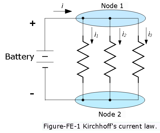
KCL states that the net current entering a node is zero.

Sum of currents into a node is equal to sum of currents leaving the node and can be expressed mathematically as

$\sum_{i=0}^N i_n=0~~~~(1.1),$ Kirchhoff’scurrent law

This is a consequence of conservation of charge * Cannot have accumulation of charge

Think of: pipes and fluid flow $\to$ water in must go out.

Kirchhoff’s current law states that because charge cannot be created but must be conserved, the sum of the currents at a node must equal zero as can be seen in Figure-FE-1.

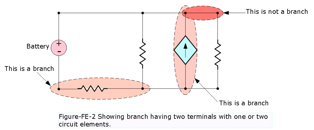
Branch:

A branch is defined to be a section of a circuit having two terminals containing one or two circuit elements as shown in Figure-FE-2.

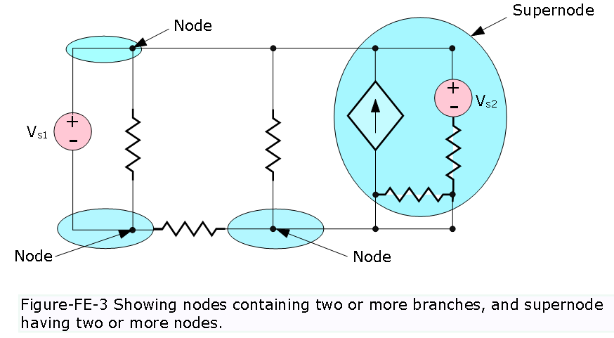
Node:

A node as illustrated in Figure-FE-3 is the junction of having two or more branches. illustrates the concept. In reality, any connection that can be made by soldering various terminals together is a node. Identifying nodes is very important for nodal analysis of electrical networks.

A supernode is obtained by defining a region that encloses more than one node. Supernodes can be considered in exactly the same way as nodes.

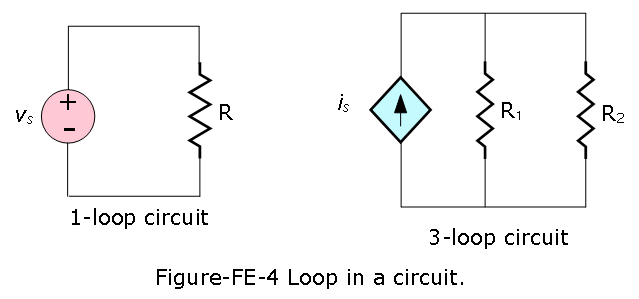
Loop:

A loop is any closed connection of branches. Various loop configurations are shown in Figure-FE-4.

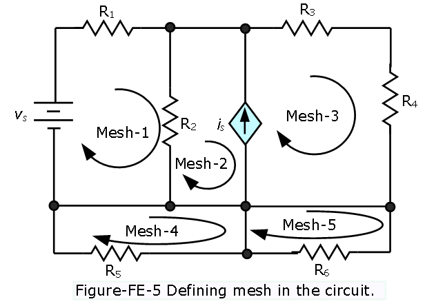
Mesh:

A mesh is a loop that does not contain other loops inside. Similar to nodes, meshes are important for mesh analysis used in network analysis. In Figure-FE-5 illustrates the meshes in a circuit.

Example-FE-1 Determine the total charge entering a circuit element between t = 1 s and t = 2 s if the current passing through the element is i = 5t.

Solution:

\[q_{total}=\int_{t_1}^{t_2}i(t)dt = \int_{t=1s}^{t=2s}5t~dt=\left[\frac {5t^2}{2}\right]_{t=1s}^{t=2s}=7.5~C~(Ans)\]

Example-FE-2 A lightbulb sees a 3-A current for 15 s. The lightbulb generates 3 kJ of energy in the form of light and heat. What is the voltage drop across the lightbulb?

Solution:

\[\Delta w = P\Delta t = vi\Delta t\] \[v=\frac{\Delta w}{i\Delta t}=\frac{3\times 10^3~J}{(3~A)(15~s)}=66.67~V~(Ans)\] Example-FE-3 How much energy does a 75-W electric bulb consume in six hours?

Solution:

\[w = Pt = (75 ~J/s)(6\times3600~s)=1.62~MJ~(Ans)\]

Example-FE-4 Find the voltage drop $v_{ab}$ required to move a charge q from point a to point b if q = −6 C and it takes 30 J of energy to move the charge.

Solution:

\[v_{ab}=\frac{w}{q}=\frac{30~J}{-6~C}=-5~V~(Ans)\] Example-FE-5 Two 2-mC charges are separated by a dielectric with thickness of 4 mm, and with dielectric constant $\epsilon = 10^{−12}$ F/m. What is the force exerted by each charge on the other?

\[F = \frac{1}{4\pi\epsilon}\frac{q_1q_2}{r^2}=\frac{1}{(4\pi\times 10^{−12}~F/m)}\frac{(2\times 10^{-3}~C)^2}{(4\times 10^{-3}~m)^2}=2\times 10^{10}~N~(Ans)\]

Example-FE-6 The magnitude of the force on a particle of charge q placed in the empty space between two infinite parallel plates with a spacing d and a potential difference V is proportional to:

qV /d2 (b) qV /d (c) qV 2/d (d) q2V/d (e) q2V2/d

Solution:

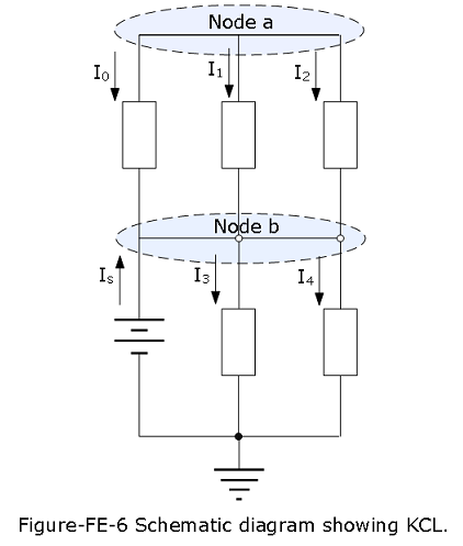
\[V = \frac{w}{q}=\frac{Fd}{q}\] \[F=\frac{qV}{d}~(Ans)\] Example-FE-7 Application of KCL: Determine the unknown currents in the circuit of Figure-FE-6. Given $I_0 = 0.5A, I_2 = 2A, I_3 = 7A, I_4 = -1A$, find $I_1$ and $I_s$.

Solution:

In Figure-FE-1 node a and node b, and the third node in the circuit is the reference (ground) node. We apply KCL at each of the three nodes.

At node a:

$I_0 + I_1 + I_2 = 0$

$0.5 + I_1 + 2 = 0$

Thus, $I_1 = -2.5A$

Note that the three currents are all defined as flowing away from the node, but but the current $I_1$ comes out to be a negative value (i.e., it is actually flowing toward the node).

At node b:

$I_S − I_3 − I_4 = 0$

$I_s - 7 -(− 1) = 0$

Thus, $I_s = 6A$

Note that the current from the battery is defined in a direction opposite to that of the other two currents. Thus, in applying KCL, we have used opposite signs for the first and the latter two currents.

At the reference node: If we use the same convention (positive value for currents entering the node and negative value for currents exiting the node), we obtain the following equations:

$−I_s + I_3 + I_4 = 0$

$−I_s + 7 - 1 = 0$

Thus, $I_s = 6A$

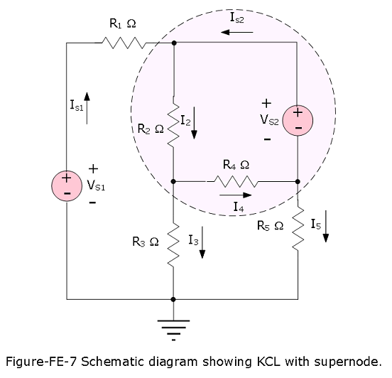
Example-FE-8 Application of KCL:Apply KCL to the circuit of Figure-FE-7, using the concept of supernode to determine the source current $I_{S1}$.Given $I_3 = 2A, I_5 = 0A$, find $I_{S1}$.

Solution:

Treating the supernode as a simple node, we apply KCL at the supernode to obtain

$I_{S1} − I_3 − I_5 = 0$

$I_{S1} = I_3 + I_5 = 2A-0A= 2A$

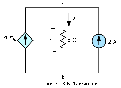
Example-FE-9:

Using KCL find the current $i_0$ and the voltage $v_0$ in the circuit shown in Figure-FE-8.

Solution:

Applying KCL to node a, we obtain

\[0.5i_0+2A = i_0\] \[i_0=10A\]

For the 5$\Omega$ resistor, Ohm’s law gives

\[v_0=i_0R=(10A)(5\Omega)=50\Omega\space (Ans)\]

Kirchhoff’s Voltage Law:

Kirchhoff’s Voltage Law (KVL):

The principle underlying KVL is that no energy is lost or created in an electric circuit; in circuit terms, the sum of all voltages associated with sources must equal the sum of the load voltages, so that the net voltage around a closed circuit is zero.

$\sum_{i=0}^N v_n=0~~~~(1.4)$, Kirchhoff’svoltage law

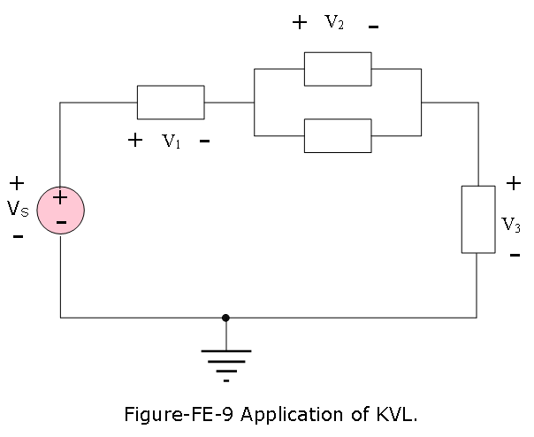
Example-FE-10: Application of KVL: Determine the unknown voltage $V_2$ by applying KVL to the circuit of Figure-FE-9. Given $V_{S} = 12 V, V_1 = 6 V, V_3 = 1 V, find~~ V_2$.

Solution:

Applying KVL around the simple loop, we write

$V_{S} − V_1 − V_2 − V_3 = 0$

$V_2 = V_{S} − V_1 − V_3 = 12 − 6 − 1 = 5 V$

Note that $V_2$ is the voltage across two branches in parallel, and it must be equal for each of the two elements, since the two elements share the same nodes.

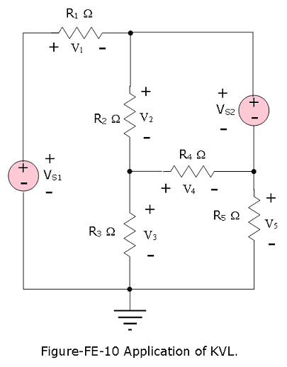
Example-FE-11: Application of KVL: Use KVL to determine the unknown voltages $V_1$ and $V_4$ in the circuit of Figure-FE-10. Given $V_{S1} = 12 V, V_{S2} = −4 V, V_2 = 2 V, V_3 = 6 V, V_5 = 12 V$, find $V_1$, $V_4$.

Solution:

Analysis: To determine the unknown voltages, we apply KVL clockwise around each of the three meshes:

$V_{S1} − V_1 − V_2 − V_3 = 0$

$V_2 − V_{S2} + V_4 = 0$

$V_3 − V_4 − V_5 = 0$

Next, we substitute numerical values:

$12 − V_1 − 2 − 6 = 0$

$V_1 = 4 V$

$2 − (−4) + V_4 = 0$

$V_4 = −6 V$

$6 − (−6) − V_5 = 0$

$V_5 = 12 V$

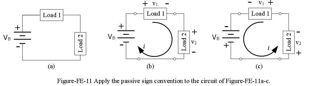
Example-FE-12: Application of KVL:Use of the Passive Sign Convention Apply the passive sign convention to the circuit of Figure-FE-11(a).Voltages across each circuit element; current in circuit. Find the power dissipated or generated by each element. Figure-FE-11(b) and (c). The voltage drop across load 1 is 8 V, that across load 2 is 4 V; the current in the circuit is 0.1 A.

Solution:

Analysis: Note that the sign convention is independent of the current direction we choose. We now apply the method twice to the same circuit. Following the passive sign convention, we first select an arbitrary direction for the current in the circuit; the example will be repeated for both possible directions of current flow to demonstrate that the methodology is sound.

Assume clockwise direction of current flow, as shown in Figure-FE-11(b), $v_B = 12 V, v_1=8V,i=0.1A,v_2=4V$.
Label polarity of voltage source, as shown in Figure-FE-11(b); since the arbitrarily chosen direction of the current is consistent with the true polarity of the voltage source, the source voltage will be a positive quantity.
Assign polarity to each passive element, as shown in Figure-FE-11(b).
Compute the power dissipated by each element: Since current flows from − to + through the battery, the power dissipated by this element will be a negative quantity:

$P_B = −v_B \times i = −12 V × 0.1A= −1.2W$

that is, the battery generates 1.2 watts (W). The power dissipated by the two loads will be a positive quantity in both cases, since current flows from plus to minus:

$P_1 = v_1 \times i = 8 V \times 0.1A = 0.8W$

$P_2 = v_2 \times i = 4 V \times 0.1A = 0.4W$

Next, we repeat the analysis, assuming counterclockwise current direction.

Assume counterclockwise direction of current flow, as shown in Figure-FE-11(c), $v_B = -12 V, v_1=-8V,i=-0.1A,v_2=-4V$.
Label polarity of voltage source, as shown in Figure-FE-11(c); since the arbitrarily chosen direction of the current is not consistent with the true polarity of the voltage source, the source voltage will be a negative quantity.
Assign polarity to each passive element, as shown in Figure-FE-11(c).
Compute the power dissipated by each element: Since current flows from plus to minus through the battery, the power dissipated by this element will be a positive quantity; however, the source voltage is a negative quantity: $P_B = v_B \times i = (−12 V)(0.1A) = −1.2W$ that is, the battery generates 1.2 W, as in the previous case. The power dissipated by the two loads will be a positive quantity in both cases, since current flows from plus to minus:

$P_1 = v_1 \times i = 8 V \times 0.1A = 0.8W$

$P_2 = v_2 \times i = 4 V \times 0.1A = 0.4W$

Comments: It should be apparent that the most important step in the example is the correct assignment of source voltage; passive elements will always result in positive power dissipation. Note also that energy is conserved, as the sum of the power dissipated by source and loads is zero. In other words: Power supplied always equals power dissipated.

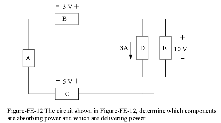
Example-FE-13: The circuit shown in Figure-FE-12, determine which components are absorbing power and which are delivering power. Is conservation of power satisfied? Explain your answer. Current through elements D and E; voltage across elements B, C, E are known which components are absorbing power, which are supplying power; verify the conservation of power.

Solution:

Analysis: By KCL, the current through element B is 5 A, to the right. By KVL, −$v_a$ − 3 + 10 + 5 = 0

Therefore, the voltage across element A is

$v_a$ = 12 V (positive at the top)

A supplies (12 V)(5 A) = 60W

B supplies (3 V)(5 A) = 15W

C absorbs (5 V)(5 A) = 25W

D absorbs (10 V)(3 A) = 30W

E absorbs (10 V)(2 A) = 20W

Total power supplied = 60W+ 15W= 75W

Total power absorbed = 25W+ 30W+ 20W= 75W

Total power supplied = Total power absorbed, so conservation of power is satisfied

Equivalent circuits

The analysis of DC circuits forms the foundation of electrical engineering. The following exercises illustrate the general type of questions that might be encountered in the FE exam.

Example-FE-14: Assuming the connecting wires and the battery have negligible resistance, the voltage across the 25$\Omega$ resistance in Figure-FE-13: is

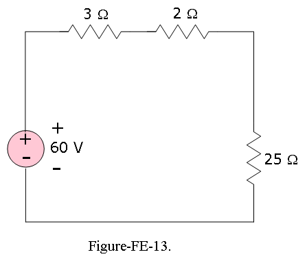
25 V b. 60 V c. 50 V d. 15 V e. 12.5 V

Solution: Using voltage divider rule, we get

\[v_{25\Omega}=60\left(\frac{25}{3+2+25}\right)=50 V\], so the answer is (c).

Example-FE-15: Assuming the connecting wires and the battery have negligible resistance, the voltage across the 6$\Omega$ resistor in Figure-FE-14: is a. 6 V b. 3.5 V c. 12 V d. 8 V e. 3 V

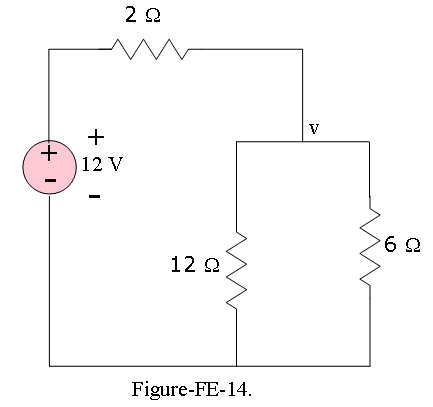
Solution: Applying nodal analysis, since one voltage is known, and applying KCL at v, we get

\[]\frac{10-v}{2}=\frac{v}{6}+\frac{v}{12}\] Solving the above equation, we get v = 8, thus the answer is (d).

Example-FE-16: In Figure-FE-15:, A 125-V battery charger is used to charge a 75-V battery with internal resistance of 1.5$\Omega$. If the charging current is not to exceed 5 A, the minimum resistance in series with the charger must be

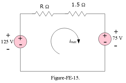
10 b. 5 c. 38.5 d. 41.5 e. 8.5

Solution: Using KVL, we get

\[i_{max}R+1.5i_{max}-125+75=0\], using $i_{max}=5A$, we get $R=8.5\Omega$,thus the answer is (e).

Capacitance and inductance:

The energy stored in the capacitor and in an inductor and their transient responses are important to understand. The exercises below briefly cover these materials.

Example-FE-17: A coil with inductance of 1 H and negligible resistance carries the current shown in Figure-FE-16:. The maximum energy stored in the inductor is

2 J b. 0.5 J c. 0.25 J d. 1 J e. 0.2 J

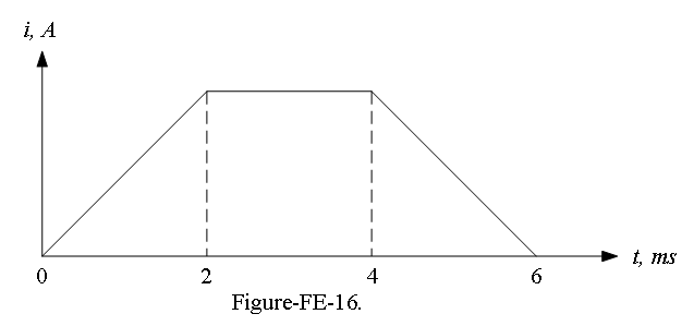
Solution:

\[W_{max}=\frac{1}{2}Li^2=\frac{1}{2}(1 H)(1A)^2=\frac{1}{2}J\], thus the answer is (b).

Example-FE-18: The maximum voltage that will appear across the coil is a. 5 V b. 100 V c. 250 V d. 500 V e. 5,000 V

Solution: The voltage across the inductor is $v=L\frac{di}{dt}.$ The slope from Figure-FE-16:,

\[\frac{di}{dt}=\frac{1}{2\times 10^{-3}}=500\] Thus, \[v_{max}=1\times 500 = 500 V\], and the answer is (d).

Example-FE-19: A voltage sine wave of peak value 100 V is in phase with a current sine wave of peak value 4 A. When the phase angle is $60^o$ later than a time at which the voltage and the current are both zero, the instantaneous power is most nearly

300W b. 200W c. 400W d. 150W e. 100W

Solution: The instantaneous AC power is

\[p(t)=\frac{VI}{2}cos\theta+\frac{VI}{2}cos(2\omega t+\theta_v+\theta_I)\] When the phase is $60^o$, later than the zero-crossing, $\theta_v=\theta_I=0$, $2\omega t = 120^o$, thus the power is

\[p=\frac{100\times 4}{2}+\frac{100\times 4}{2}cos120^o=300 W\], thus the answer is (a).

Example-FE-20: A sinusoidal voltage whose amplitude is 20$\sqrt2$ V is applied to a 5-$\Omega$ resistor. The root mean-square value of the current is

5.66 A b. 4 A c. 7.07 A d. 8 A e. 10 A

Solution:

\[V_{rms}=\frac{V}{\sqrt{2}}=\frac{20\sqrt 2 V}{\sqrt{2}}=20V\] \[I_{rms}=\frac{V_{rms}}{R}=\frac{20}{5}=4 A\], thus the answer is (b).

Example-FE-21: The magnitude of the steady-state root-mean-square voltage across the capacitor in the circuit of Figure-FE-17: is

30 V b. 15 V c. 10 V d. 45 V e. 60 V

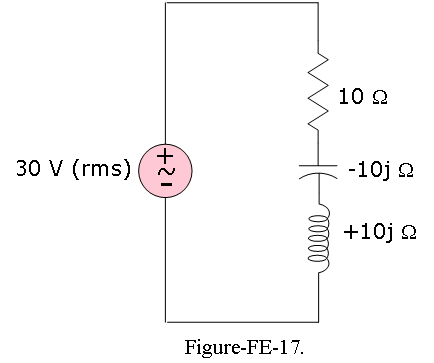
Solution:

Using the voltage divider rule for impedances, the voltage across the capacitor is

\[V=30\angle 0^o\times\frac{-j10}{10-j10+j10}=30\angle 0^o\times(-j1)=30\angle 0^o\times 1\angle -90^o=30\angle 90^o\] Thus, the root-mean-square voltage across the capacitor is 30 V, and is therefore the answer is (a).

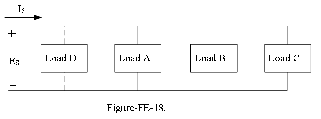
The next set of questions (Example-FE-44 to 48) pertain to single-phase AC power calculations and refer to the single-phase electrical network shown in Figure-FE-18:. In this figure, $E_S = 480\angle 0^o$ V; $I_S = 100\angle -15^o$ A; $\omega = 120\pi$ rad/s. Further, load A is a bank of single-phase induction machines. The bank has an efficiency $\eta$ of 80 percent, a power factor of 0.70 lagging, and a load of 20 hp. Load B is a bank of overexcited single-phase synchronous machines.The machines draw 15 kVA, and the load current leads the line voltage by $30^o$. Load C is a lighting (resistive) load and absorbs 10 kW. Load D is a proposed single-phase capacitor that will correct the source power factor to unity. This material is covered in Sections 7.1 and 7.2.

Example-FE-22: The root-mean-square magnitude of load A current, denoted by $I_A$, is most nearly

44.4 A b. 31.08 A c. 60 A d. 38.85 A e. 55.5 A

Solution: The output power $P_o$ of a single phase induction motor $P_0=(20 hp)(746 W/hp)=14,920 W$. The input electric power is

\[P_{in}= \frac{P_0}{\eta}=\frac{14,920 W}{0.80}=18,650 W\] Also, \[P_{in}=E_SI_Acos\theta_A\] \[I_A=\frac{P_{in}}{E_Scos\theta_A}=\frac{18,650 W}{480\times 0.70}\approx55.5 A\]. Thus, the answer is (e).

Example-FE-23: The phase angle of $I_A$ with respect to the line voltage $E_S$ is most nearly

$a. 36.87^o~~ b. 60^o ~~c. 45.6^o~~ d. 30^o~~ e. 48^o$

Solution:

The phase angle $I_A$ and $E_S$ is \[\theta = cos^{-1}(-0.70)=45.57^o\approx 45.6^o\], thus the answer is (c).

Example-FE-24: The power absorbed by synchronous machines is most nearly

20,000W b. 7,500W c. 13,000W d. 12,990W e. 15,000W

Solution:

The apparent power S is given to be 15 kVA, and $\theta=30^o$. The power drawn by the bank of synchronous motors is

P = $Scos\theta$ = $15,000\times \cos30^o=12,990.38 W=12.99kW$, thus the answer is (d).

Example-FE-25: The power factor of the system before load D is installed is most nearly

0.70 lagging b. 0.866 leading c. 0.866 lagging d. 0.966 leading e. 0.966 lagging

Solution:

pf = $cos15^o=0.966$ lagging, thus the answer is (e).

Example-FE-26: The capacitance of the capacitor that will give a unity power factor of the system is most nearly

219 $\mu F$ 4 b. 187 $\mu F$ c. 132.7 $\mu F$ d. 240 $\mu F$ e. 132.7 pF

Solution:

The reactive power $Q_A$ in load A is \[Q_A = P_A\times tan\theta_A\] \[\theta_A=cos^{_1}0.70=45.57^O\] \[Q_A=18.65\times45.57^o=19,025VAR\] The total reactive power $Q_B$ in load B is \[Q_B=5\times sin\theta_B=15,000\times sin(-30^o)=-7,500VAR\] The total reactive power Q is \[Q=Q_A+Q_B=19,025-7,500=11,525VAR\] To cancel this reactive power, we set \[Q_C=-Q= -11,525VAR\] \[Q_C=-\frac{E_S^2}{X_C}\] and \[X_C=-\frac{1}{\omega C}\] \[C=-\frac{Q_C}{\omega E_S^2}=\frac{11,525}{120\pi\times 480^2}=132.7\mu F\], thus the answer is (c).

Reactance and impedance, susceptance and admittance:

Example-FE-27: Given the $C_1 = 0.001 \mu F$ = $1 \times 10^{−9}$ F; $R_1 = 1 M\Omega$ as shown in Figure-FE-19. Find the equivalent impedance of the parallel circuit $Z_1$.Find the impedance of a practical capacitor at the radian frequency $\omega$ = 377 rad/s (60 Hz). How will the impedance change if the capacitor is used at a much higher frequency, say, 800 kHz?

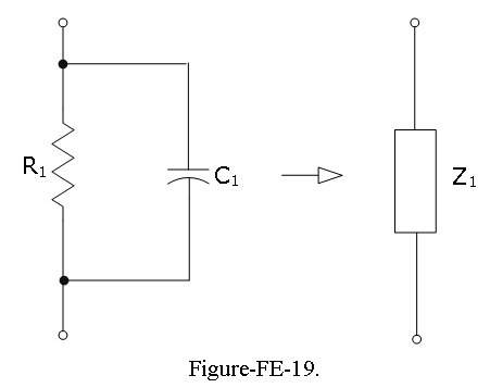
Solution:

\[\frac{1}{Z_1}=\frac{1}{R_1}+j\omega C_1\] \[Z_1(\omega)=\frac{R_1}{1+j\omega C_1 R_1}\] \[Z_1(\omega=377 ~rad/s)=\frac{1\times 10^6~\Omega}{1+j(377~rad/s) 10^{-9}\times 10^6\Omega}=\frac{1\times 10^6}{1+j0.377}=9.3571\times 10^5\angle\] \[Z_1(\omega=377 ~rad/s)=\frac{1\times 10^6}{1+j0.377}=\frac{1\times 10^6(1-j0.377)}{\sqrt{1^2+(0.377)^2}}= 9.3571\times 10^5\angle (-0.3605)~\Omega\] The impedance of the capacitor alone at this frequency would be \[Z_{C1}(\omega = 377~rad/s)=\frac{1}{j\omega C_1}=\frac{1}{j377\times 10^{-9}}=2.6525\times 10^5\angle (-\frac{\pi}{2})~\Omega\] You can easily see that the parallel impedance $Z_1$ is quite different from the impedance of the capacitor alone, $Z_{C1}$.

If the frequency is increased to 800 kHz, or $1600\pi \times 10^3$ rad/s, a radio frequency in the AM range then we can recompute the impedance to be

\[Z_1(\omega)=\frac{R_1}{1+j\omega C_1 R_1}\] \[Z_1(\omega=377 ~rad/s)=\frac{1\times 10^6~\Omega}{1+j(377~rad/s) 10^{-9}\times 10^6\Omega}=\frac{1\times 10^6}{1+j0.377}=9.3571\times 10^5\angle\] \[Z_1(\omega=1600\pi\times 10^3 ~rad/s)=\frac{1\times 10^6}{1+j1600\pi\times10^3\times10^{-9}\times 10^6}=\frac{10^6}{1+j1600\pi}=198.9\angle(-1.5706)~|Omega\] The impedance of the capacitor alone at this frequency would be \[Z_{C1}(\omega = 1600\pi\times 10^3~rad/s)=\frac{1}{j1600\pi\times 10^3\times 10^{-9}}=198.9\angle(-\pi/2)~\Omega\] Now, the impedances $Z_1$ and $Z_{C1}$ are virtually identical (note that $\pi/2$ = 1.5708 rad). Thus, the effect of the parallel resistance is negligible at high frequencies.

Comments: The effect of the parallel resistance at the lower frequency (corresponding to the well-known 60-Hz AC power frequency) is significant: The effective impedance of the practical capacitor is substantially different from that of the ideal capacitor. On the other hand, at much higher frequency, the parallel resistance has an impedance so much larger than that of the capacitor that it effectively acts as an open circuit, and there is no difference between the ideal and practical capacitor impedances. This example suggests that the behavior of a circuit element depends very much on the frequency of the voltages and currents in the circuit.

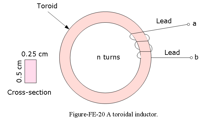
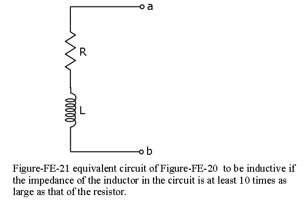
Example-FE-28: A practical inductor can be modeled by an ideal inductor in series with a resistor with the given L = 0.098 H; lead length = $l_c = 2 \times 10 cm$; n = 250 turns; wire is 30-gauge. Resistance of 30-gauge wire = $0.344 ~\Omega/m$. Figure-FE-20 shows a toroidal (doughnut-shaped) inductor. The series resistance represents the resistance of the coil wire and is usually small. Find the range of frequencies over which the impedance of this practical inductor is largely inductive (i.e., due to the inductance in the circuit). We shall consider the impedance to be inductive if the impedance of the inductor in the circuit of Figure-FE-21 is at least 10 times as large as that of the resistor.

Solution:

We first determine the equivalent resistance of the wire used in the practical inductor, using the cross section as an indication of the wire length $l_w$ in the coil:

$l_w$ = 250(2 × 0.25 + 2 × 0.5) = 375 cm

$l$ = total length = $l_w$ + $l_c$ = 375 + 20 = 395 cm

The total resistance is therefore R = 0.344 $\Omega$/m × 0.395 m = 0.136$\Omega$

Thus, we wish to determine the range of radian frequencies, $\omega$, over which the magnitude of $j\omega L$ is greater than 10 × 0.136 $\Omega$:

$ωL \gt 1.36$ or $ = = 1.39 rad/s

Alternatively, the range is $f = \frac{\omega}{2\pi} \gt 0.22$ Hz.

Comments: Note how the resistance of the coil wire is relatively insignificant. This is true because the inductor is rather large; wire resistance can become significant for very small inductance values. At high frequencies, a capacitance should be added to the model because of the effect of the insulator separating the coil wires.

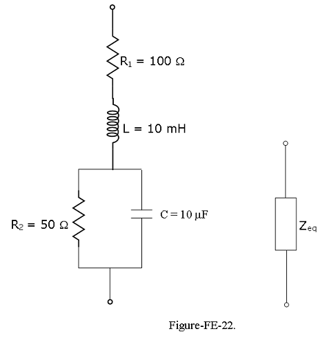
Example-FE-29: Given the $\omega = 10^4$ rad/s; $R_1$ = 100 $\Omega$; L = 10 mH; $R_2$ = 50 $\Omega$; C = 10 $\mu$ F. Find the equivalent impedance of the circuit shown in Figure-FE-22 with a more complex circuit.

Solution:

We determine first the parallel impedance $Z_{||}$ of the $R_2-C$ circuit.

\[\frac{1}{Z_{||}}=\frac{1}{R_2}+j\omega CR_2=\frac{1+j\omega CR_2}{R_2}\] \[Z_{||}=\frac{R_2}{1+j\omega CR_2}=\frac{50\Omega}{1+j(10^4~ rad/s)(10\times 10^{-6}F)(50 \Omega)}=\frac{50}{1+j5}=1.92-j9.62=9.81\angle -(1.3734)\] \[Z_{||}==1.92-j9.62=9.81\angle -(1.3734)\Omega\] Next, we determine the equivalent impedance $Z_{eq}$:

\[Z_{eq}=R_1+j\omega L+Z_{||}=100+j10^4\times 10^{-2}+1.92-j9.62\] \[Z_{eq}=101.92+j90.38=136.2\angle 0.723\Omega\] Is this impedance inductive or capacitive? At the frequency used in this example, the circuit has an inductive impedance, since the reactance is positive (or, alternatively, the phase angle is positive).

Admittance:

The admittance of a branch is defined as follows:

\[Y=\frac{1}{Z}~~~S\] Note immediately that whenever Z is purely real, that is, when Z = R + j0, the admittance Y is identical to the conductance G. In general, however, Y is the complex number

\[Y = G + jB\] where G is called the AC conductance and B is called the susceptance; the latter plays a role analogous to that of reactance in the definition of impedance. Clearly, G and B are related to R and X . However, this relationship is not as simple as an inverse. Let Z = R + jX be an arbitrary impedance. Then the corresponding admittance is

\[Y=\frac{1}{Z}=\frac{1}{R+jX}\] To express Y in the form Y = G + jB, we multiply numerator and denominator by R − jX:

\[Y=\frac{1}{R+jX}\frac{R-jX}{R-jX}=\frac{R-jX}{R^2+X^2}=\frac{R}{R^2+X^2}-j\frac{X}{R^2+X^2}\] and thus

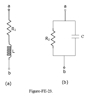
\[G = \frac{R}{R^2+X^2}\] and \[B=-\frac{X}{R^2+X^2}\] Example-FE-30: Given $\omega = 2\pi\times 10^3$ rad/s; $R_1 = 50 ~\Omega$; L = 16 mH; $R_2 = 100~$; $C = 3~ \mu F$. Find the equivalent admittance of the two circuits shown in Figure-FE-23.

Solution:

Circuit (a): First, determine the equivalent impedance of the circuit:

\[Z_{ab} = R_1 + j\omega L\] Then compute the inverse of $Z_{ab}$ to obtain the admittance:

\[Y_{ab}=\frac{1}{R_1+j\omega L}=\frac{R_1-j\omega L}{R_1^2+\omega^2L^2}\] Substituting the values of the given parameters gives

\[Y_{ab}=\frac{1}{50+j2\pi\times 10^3\times 0.016}=\frac{1}{50+j100.5}=3.968\times10^{-3}-j7.976\times 10^{-3}~S\] Circuit (b): First, determine the equivalent impedance of the circuit:

\[Z_{ab}=R_2{\parallel}\frac{1}{j\omega C}=\frac{R_2}{j\omega CR_2}\]

Then compute the inverse of $Z_{ab} to obtain the admittance:

\[Y_{ab}=\frac{1+j\omega CR_2}{R_2}=\frac{1}{R_2}+j\omega C=0.01+j0.019~~S\]

Note that the units of admittance are siemens (S), that is, the same as the units of conductance.

AC circuits:

The material related to basic AC circuits is covered in Chapter 4, sections 2 and 4. Examples 4.8, 4.9, 4.16, 4.17, 4.18, 4.19, 4.20, 4.21, and the related materials. In addition, material on AC power may be found in Chapter 7, Sections 1 and 2. Examples 7.1 through 7.11 and the accompanying

Average and RMS Values:

Example-FE-31: Compute the average value of the signal x(t) = 10 cos(100t).

Solution: The signal is periodic with period T = $2\pi/\omega = 2\pi/100$; thus we need to integrate over only one period to compute the average value:

\[<x(t)>=\frac{1}{T}\int_0^Tx(t')dt'=\frac{100}{2\pi}\int_0^{2\pi/00}10cos(100t)dt=\frac{10}{2\pi}<sin(2\pi)-sin(0)>=0\] Comments: The average value of a sinusoidal signal is zero, independent of its amplitude and frequency.

Example-FE-32: Compute the rms value of the sinusoidal current i(t) = I $cos(\omega t)$.

Solution: Applying the definition of rms value, we compute

\[i_{rms}=\sqrt{\frac{1}{T}\int_0^Ti^2(t')dt'}=\sqrt{\frac{\omega}{2\pi}\int_0^{2\pi/\omega}I^2cos^2(\omega t')dt'}\] \[=\sqrt{\frac{\omega}{2\pi}\int_0^{2\pi/\omega}I^2\left[\frac{1}{2}+\frac{1}{2}cos(2\omega t')\right]dt'}\] \[=\sqrt{\frac{1}{2}I^2+\frac{\omega}{2\pi}\int_0^{\frac{2\pi}{\omega}}\frac{I^2}{2}cos(2\omega t')dt'}\] At this point, we recognize that the integral under the square root sign is equal to zero, because we are integrating a sinusoidal waveform over two periods.

Hence, \[i_{rms} = \frac{I}{\sqrt{2}} = 0.707I\] where I is the peak value of the waveform i(t).

Comments: The rms value of a sinusoidal signal is equal to 0.707 times the peak value, independent of its amplitude and frequency.

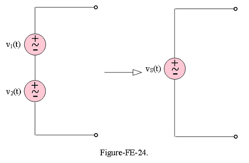
Example-FE-33: Given $v_1(t) = 15cos(377t+\pi/4)$ and $v_2(t) = 15cos(377t+\pi/12)$ find the equivalent phasor voltage $v_S(t)$. Compute the phasor voltage resulting from the series connection of two sinusoidal voltage sources as shown in Figure-FE-24.

Solution:

Given $v_1(t) = 15cos(377t+\pi/4)$ and $v_2(t) = 15cos(377t+\pi/12)$

The corresponding two voltages in phasor form:

\[V_1(j\omega)=15\angle \pi/4~~~V\] \[V_2(j\omega)=15\angle \pi/12~~~V\] Convert the phasor voltages from polar to rectangular form:

\[V_1(j\omega)=10.61+j10.61~~~V\] \[V_1(j\omega)=14.49+j3.88~~~V\] Thus

\[V_S(j\omega) = V_1(j\omega) + V_2(j\omega) =25.10+j14.49=28.98\angle \pi/6~~~V\] Now we can convert $V_S(j\omega)$ to its time-domain form:

\[v_S(t)=28.98cos(377t+\pi/6)~~~V\]

Superposition of AC Signals:

The circuit shown in Figure-FE-25 depicts a source excited by two current sources connected in parallel, where

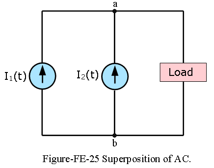
\[i_1(t) = A_1cos(\omega_1t)\] \[i_2(t) = A_2cos(\omega_2t)\] The load current is equal to the sum of the two source currents; that is,

\[i_L(t) = i_1(t) + i_2(t)\] or, in phasor form,

\[I_L = I_1 + I_2\]

Example-FE-34: Given the $i_S(t) = 0.5cos[2\pi(100t)]$ A and $v_S(t) = 20 cos[2\pi(1,000t)]$ V as shown in Figure-FE-26, compute the voltages $v_{R1}(t)$ and $v_{R2}(t)$ using the method of superposition.

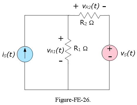
Solution:

Since the two sources are at different frequencies, we must compute a separate solution for each. Consider the current source first, with the voltage source set to zero (short circuit) as shown in Figure-FE-27. The circuit thus obtained is a simple current divider. Write the source current in phasor notation:

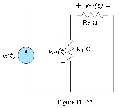
\[I_S(jomega0=0.5e^{j0}=0.5\angle 0~~~A; ~~\omega=2\pi (100)~rad/s\] Then, \[V_{R1}(I_S)=I_S\frac{R_2}{R_1+R_2}R_1=0.5\angle 0(\frac{50}{150+50})150=18.75\angle0~~V; ~~\omega=2\pi(100)~rad/s\] \[V_{R2}(I_S)=I_S\frac{R_1}{R_1+R_2}R_2=0.5\angle 0(\frac{150}{150+50})50=18.75\angle0~~V; ~~\omega=2\pi(100)~rad/s\] Next, we consider the voltage source, with the current source set to zero (open circuit), as shown in Figure-FE-28. We first write the source voltage in phasor notation:

\[V_{R1}(V_S)=V_S\frac{R_2}{R_1+R_2}R_1=20\angle 0(\frac{50}{150+50})150=15\angle0~~V; ~~\omega=2\pi(100)~rad/s\] \[V_{R2}(V_S)=-V_S\frac{R_1}{R_1+R_2}R_2=-20\angle 0(\frac{150}{150+50})50=-5\angle\pi~~V; ~~\omega=2\pi(100)~rad/s\] Now we can determine the voltage across each resistor by adding the contributions from each source and converting the phasor form to time-domain representation:

\[V_{R1} = V_{R1}(I_S) + V_{R1}(V_S)\]

\[v_{R1}(t) = 18.75 cos[2\pi(100t)] + 15 cos[2\pi(1,000t)]~~V\]

and

\[V_{R_2} = V_{R2}(I_S ) + V_{R2}(V_S)\]

\[v_{R2}(t) = 18.75 cos[2\pi(100t)] + 5 cos[2\pi(1,000t) + \pi]~~V\]

Note that it is impossible to simplify the final expression any further because the two components of each voltage are at different frequencies.

AC Power:

In this section the students are expected to learn how to calculate the AC power and the process of generation and distribution of electric power.

The topic of electric power is based on the subject materials developed in the previous sections, such as phasors and complex impedance that will lead to the electric machines.

Also, students will learn how to calculate the power factor,power factor correction,an ideal transformers, maximum power transfer, an introduction to three-phase power, and finally to power generation and distribution.

Instantaneous and Average Power:

In a linear electric circuit is excited by a sinusoidal source, all voltages and currents in the circuit are also sinusoids of the same frequency as that of the excitation source.

Figure-FE-29 shows the general form of a linear AC circuit.

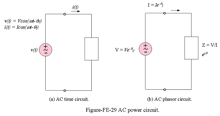
The most general expressions for the voltage and current delivered to an arbitrary load are as follows:

\[v(t) = Vcos(\omega t −\theta_V)\] \[i(t) = I cos(\omega t − \theta_I )\]

where V and I are the peak amplitudes of the sinusoidal voltage and current, respectively, and $θ_V$ and $θ_I$ are the respective phase angles. Two such waveforms are plotted in Figure-FE-30, with unit amplitude and with phase angles $\theta_V = \pi/6$ and $\theta_I = \pi/3$.

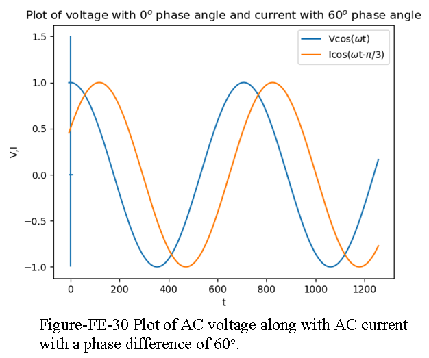
The phase shift between source and load is therefore $\theta = \theta_V − \theta_I$. For simplicity, we assume that $\theta_V$ = 0, without any loss of generality, since all phase angles will be referenced to the source voltage’s phase.

The instantaneous power dissipated by a circuit element is given by the product of the instantaneous voltage and current, it is possible to obtain a general expression for the power dissipated by an AC circuit element:

\[p(t) = v(t)i(t) = VI cos(\omega t)cos(\omega t − \theta)\] Using trigonometric identities to yield

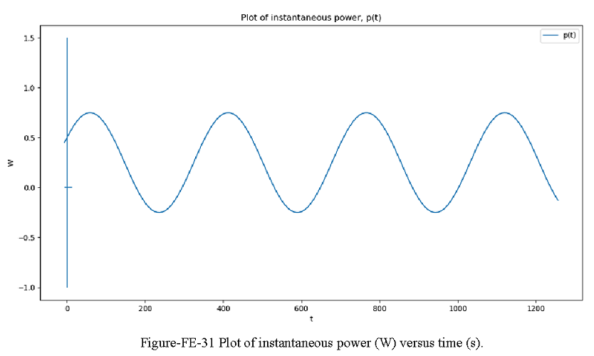
\[p(t) = \frac{VI}{2}cos(\theta) + \frac{VI}{2}cos(2\omega t − \theta)\] where $theta$ is the difference in phase between voltage and current. This equation illustrates how the instantaneous power dissipated by an AC circuit element is equal to the sum of an average component $\frac{1}{2}VIcos(\theta)$ and a sinusoidal component $\frac{1}{2}VIcos(2\omega t −\theta)$, oscillating at a frequency double that of the original source frequency.

The instantaneous and average power are plotted in Figure-FE-31 for the signals of Figure-FE-30. The average power corresponding to the voltage and current can be obtained by integrating the instantaneous power over one cycle of the sinusoidal signal. Let $T = 2\pi/\omega$ represent one cycle of the sinusoidal signals.

Then the average power $P_{av}$ is given by the integral of the instantaneous power p(t) over one cycle

\[P_{av}=\frac{1}{T}\int_0^Tp(t)dt=\frac{1}{T}\int_0^T\frac{VI}{2}cos(\theta)dt+\frac{1}{T}\int_0^T\frac{VI}{2}cos(2\omega t-\theta)dt=\frac{VI}{2}cos(\theta)\] since the second integral is equal to zero and $cos(\theta)$ is a constant. In phasor notation, the current and voltage are given by

\[V(j\omega) = Ve^{j0}\] \[I(j\omega) = Ie^{−j\theta}\] The impedance of the circuit element is defined by the phasor voltage and current to be

\[Z = \frac{V}{I}e^{j(\theta)} = |Z|e^{j\theta}\] The expression for the average power using phasor notation, as follows:

\[Pav = \frac{1}{2}\frac{V^2}{|Z|} cos \theta = \frac{1}{2} I^2|Z|cos\theta\]

An AC power systems operate at a fixed frequency; in North America, this frequency is 60 cycles per second, or hertz (Hz), corresponding to a radian frequency

$\omega = 2\pi· 60$ = 377 rad/s AC power frequency

In Europe and most other parts of the world, AC power is generated at a frequency of 50 Hz as a result some of the appliances will not operate under one of the two systems.

In AC power analysis the rms value of the AC voltages and currents in the circuit eliminates the factor 1/2 in power expressions. Thus, the following expressions will be used in the rest of the discussions:

$V_{rms}=\frac{V}{\sqrt2}=\tilde{V}$; $I_{rms}=\frac{I}{\sqrt2}=\tilde{I}$;

\[P_{av}=\frac{1}{2}\frac{V^2}{|Z|cos\theta}=\frac{\tilde{V}^2}{|Z|}cos\theta\] \[P_{av}=\frac{1}{2}I^2|Z|cos\theta=\tilde{I}^2{|Z|}cos\theta=\tilde{V}\tilde{I}cos\theta\] Figure-FE-32 illustrates the impedance triangle, which provides a convenient graphical interpretation of impedance as a vector in the complex plane. From the figure, it is simple to verify that

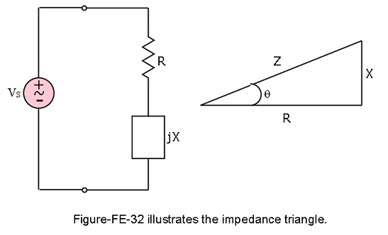
\[R = |Z| cos\theta\] \[X = |Z| sin \theta\] The amplitudes of phasor voltages and currents will be denoted throughout this chapter by means of the rms amplitude.We therefore introduce a slight modification in the phasor notation of Chapter 4 by defining the following rms phasor quantities:

\[\tilde{V}= V_{rms}e^{jθ_V} = \tilde{V}e^{jθ_V} = \tilde{V}\angle\theta_V\] and

\[\tilde{I}= I_{rms}e^{jθ_I} = \tilde{I}e^{jθ_I} = \tilde{I}\angle\theta_I\] In other words,the symbols $\tilde{V}$ and $\tilde{I}$ will denote the rms value of a voltage or a current, and the symbols $\tilde{\bf{V}}$ and $\tilde{\bf{I}}$ will denote rms phasor voltages and currents.

Thus, the sinusoidal waveform corresponding to the phasor current $\tilde{\bf{I}} = \tilde{I}\angle \theta_I$ corresponds to the time-domain waveform

\[i(t) = \sqrt{2}\tilde{I} cos(\omega t + \theta_I)\]

and the sinusoidal form of the phasor voltage $\tilde{\bf{V}} = \tilde{V}\angle \theta_V$ is

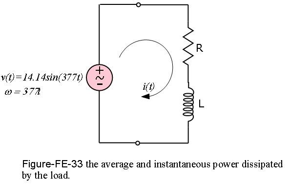
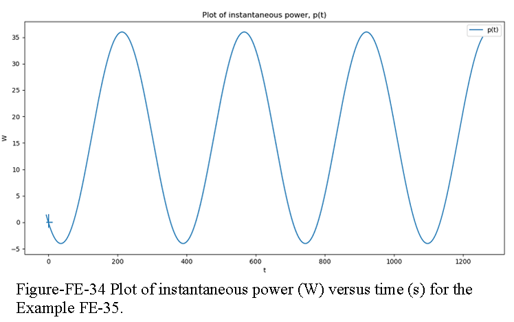
\[v(t) = \sqrt{2}\tilde{V} cos(\omega t + \theta_V)\] Example-FE-35: Given v(t) = 14.14 sin(377t) V; R = 4$\Omega$;L = 8 mH, compute the average and instantaneous power dissipated by the load of Figure-FE-33.

Solution:

The phasors and impedances at the frequency of interest in the problem, $\omega$ = 377 rad/s:

\[\tilde V = 10\angle\left(-\frac{\pi}{2}\right); Z = R+j\omega L=4+j3=5\angle0.644\] \[\tilde I=\frac{\tilde V}{Z}=\frac{10\angle(-\pi/2)}{5\angle 0.644}=2\angle (-2.215)\]

The average power can be computed from the phasor quantities:

\[P_{av}=\tilde V \tilde I cos\theta = 10\times2\times cos(\theta)=16~W\] The instantaneous power is given by the expression

\[p(t)=v(t)\times i(t) = \sqrt 2\times 10 sin(377t)\times\sqrt 2\times2cos(377t-2.215)~W\]

The instantaneous voltage and current waveforms and the instantaneous and average power are plotted in Figure-FE-34.

to be continued…….